1. Genomics

1.1 Gene search

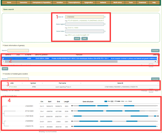
The Gene search page provides gene structure and function information of Liuyejingui genomes. In this module, the user can enter the gene ID of Liuyejingui to query the related information of the interest gene. If users entered the gene ID or gene name of Arabidopsis thaliana, the structure and function information of all homologous genes and their phylogenetic relationship can be obtained. For example, if users entered ' AT1G02970' (box1), users can obtain the physical location and functional description information of all homologous genes corresponding to this gene, the phylogenetic relationship of homologous genes.

1.2 Gene cluster

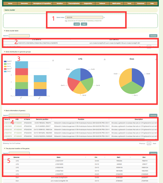
Gene cluster provides a query of gene cluster results for 2 Osmanthus genomes. The user can query the copy number of the genes by entering the Arabidopsis Gene ID or Gene name. For example, if users entered 'AT1G02400' at box1, results in boxes 2-5 will be obtained. The gene IDs of different genome assemblies corresponding to the gene cluster where the gene is located can be obtained in box2; the copy number difference of the gene cluster in all genomes is listed in box3; the functional description of the genes in this gene cluster is given in box4; the physical location information of the genes in this gene cluster will be obtained in box5.

1.3 Gene family

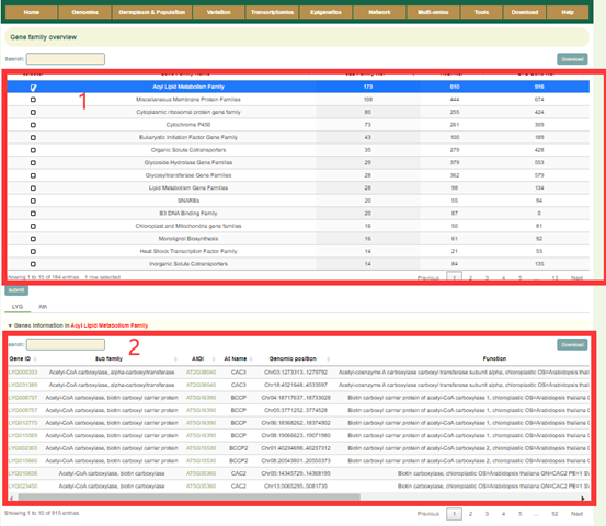
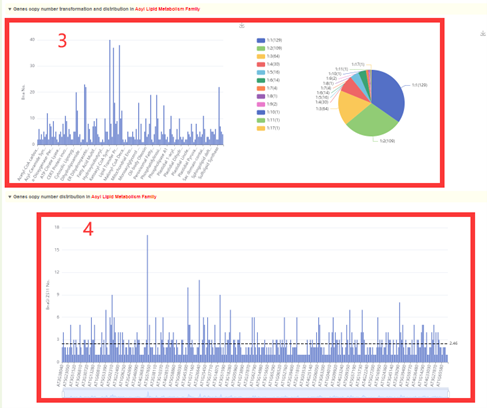
Gene family integrates information from 184 gene families. The gene number of each gene family is listed in Gene family overview(box1). Check the box in the first column to submit to view the gene list of the corresponding gene family and the statistics of the copy number of Osmanthus fragrans genome corresponding to the Arabidopsis genes in this family(box2, 3 and 4).

1.4 Gene index

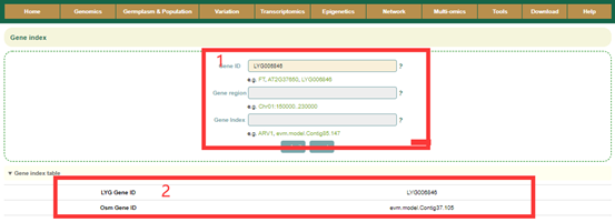
Gene index constructed a total of 13,730 gene indexes by integrating the gene collinearity of 2 Osmanthus fragrans genomes. By entering the Arabidopsis gene ID, gene name or the gene ID of the Osmanthus fragrans (box1), users can view the gene index of related genes (box2).

1.5 Genome synteny

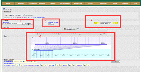
Users can browse the alignment results of all regions between genomes using Gbrowser_syn. In Gbrowser, the user selects the object of the gene alignment to view(box1), and then gets the result(box4). The genomic collinearity (box4) is finally obtained by selecting the reference genome(box2), the genomic region to be viewed(box4), and the resolution(box3).

1.6 Pathway

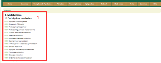
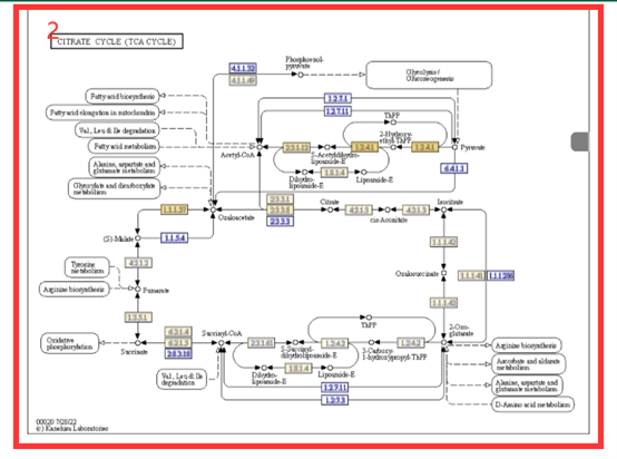
In the Pathway module, we integrated the pathway information of Liuyejingui genomes. The user can select the number of the pathway and clicking, you can get the result(box2). The boxes with different colors indicate the number of genes corresponding to different metabolites in this genome(box2). By hovering the mouse over the box1, you can view the list of genes related to the metabolite.

1.7 Transcription factor(TF)

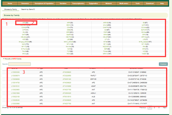
In Transcription factor module, we annotated a total of 5,956 genes encoding transcription factors in 56 families based on the TF information in the Arabidopsis genome and the homologous gene relationship between Liuyejingui and Rixianggui genomes. Users can browse the number of genes in all gene families using "Browse by Family" (box 1), and view the number of genes in that family by clicking on the gene family name. For example, when you click on AP2 (box 2), you will get a list of genes belonging to this family (box 3). In addition, users can also enter the gene ID in "Search by Gene ID" to check whether the gene is a transcriptome factor and its gene family information.

1.8 About

In the "genomics" module, we collected two published O. fragrans genomes "Liuyejingui" ^[1] and "Rixianggui" ^[2] and annotated the gene function, domains, metabolic pathways of genes in each genome. The gene ID, position, function annotation and homologous in Arabidopsis thaliana can be obtained in "Gene search" module. Totally, 86,794 genes of 2 O. fragrans genome assemblies were used to construct the gene index. Gene synteny of every pairs from 2 genome assemblies were detected by McScanX ^[3]. Gene cluster were generated based on the homologous with Arabidopsis thaliana. The "Gene family" module provided the detail gene family information of 13,730 genes in "Liuyejingui" reference genome.

We also added the interactive Scalable Vector Graphics (SVG) to exploring genes involved in different KEGG pathway (https://www.genome.jp/kegg/). Genomic synteny was constructed based on the genome alignment using Mummer, user can browse local alignment by GBrowser ^[4]. According to the PlantTFDB ^[5], the information of 56 TF families in "Liuyejingui" reference genome is provided in "Transcription factor (TF)" module.

References

1. Chen H, Zeng X, Yang J, Cai X, Shi Y, Zheng R, et al. Whole-genome resequencing of Osmanthus fragrans provides insights into flower color evolution. Hortic Res 2021, 8:98.
2. Yang X, Yue Y, Li H, Ding W, Chen G, Shi T, et al. The chromosome-level quality genome provides insights into the evolution of the biosynthesis genes for aroma compounds of Osmanthus fragrans. Hortic Res 2018, 5:72.
3. Wang Y, Tang H, Debarry JD, Tan X, Li J, Wang X, et al. MCScanX: a toolkit for detection and evolutionary analysis of gene synteny and collinearity. Nucleic Acids Res 2012, 40:e49-e49.
4. McKay SJ, Vergara IA, Stajich JE. Using the Generic Synteny Browser (GBrowse_syn). Curr Protoc Bioinformatics 2010, Chapter 9:Unit 9 12.
5. Jin J, Tian F, Yang DC, Meng YQ, Kong L, Luo J, et al. PlantTFDB 4.0: toward a central hub for transcription factors and regulatory interactions in plants. Nucleic Acids Res 2017, 45:D1040-D1045.

2. Germplasm & population

2.1 Germplasm

2.2 Population information

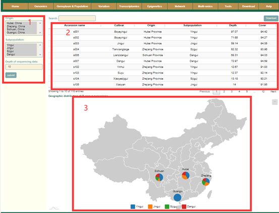
In the Population information module, users can query the related information of the collected 127 Osmanthus fragrans accessions. Users can filter accessions according to their Origin, Subpopulation, Resource, and sequencing depth (box1). Then, the user will get information such as germplasm name, geographic origin, subgroup, sequencing depth, and data source of these accessions (box 2), as well as the proportion of accessions from different subpopulations on each continent (box 3).

2.3 Population structure

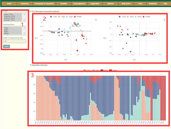
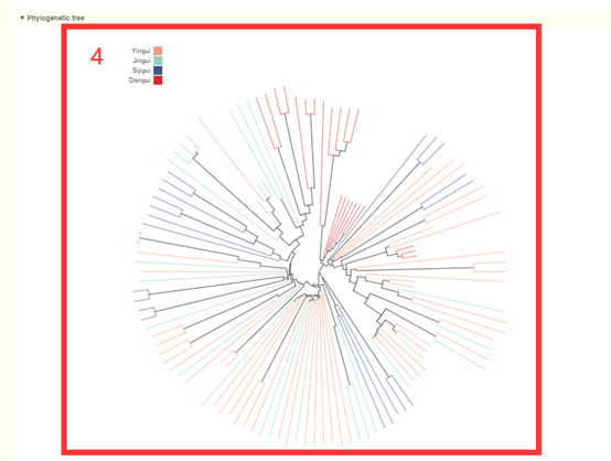
In the Population structure module, users can query the population structure information of the 119 Osmanthus fragrans accessions. Users can filter accessions according to their Origin, Subpopulation, Resource, and sequencing depth (box1). Then, users can obtain the results of PCA (box2), population structure analysis, and phylogenetic analysis of these accessions (box 3 and 4). The user can move the mouse over these points or columns to query the population structure information of this accession.

2.4 Selective signals

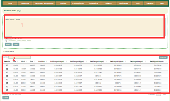
In the FST module, the user can submit the gene ID or genomic region in the search box(box 1), and then clicks “submit” to submit. Then, the FST values (box 2) and visualization results (box 3, box 4) in the area will be showed. The lines with different colors in the figure represent the FST values of the pairwise comparison between the three ecotypes. Users can also change this region on the left side of the page (box 3).

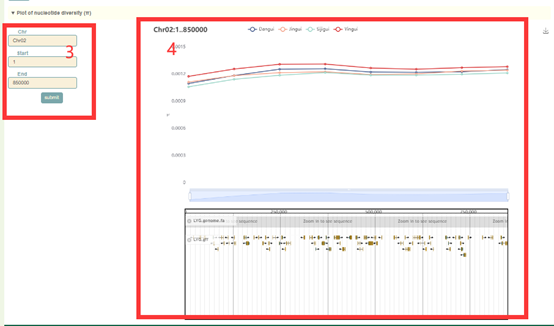
The usage of the Pi module is similar to that of FST. The user first submits the gene ID or genomic region (box 1) to query in the search box, and clicks “submit” to submit. Then, the Pi values (box 2) and visualization results (box 3, box 4) of all windows (50 kb) will be obtained. Users can also change this region on the left side of the page (box 3).

2.5 About

The "population" module includes 161 O. fragrans plant accessions from china, we provide the cultivar, geographic distribution, subgroup, and depth and coverage of resequencing for each plant. The 161 O. fragrans accessions were categorized into four subgroups: 73 "Yingui" group, 38 "Jingui" group, 22 "Sijigui" group, and 28 "Dangui" group and distributed in four regions of China: 6 Guangxi province, 19 Hubei province, 45 Sichuan province, and 48 Zhejiang province. The average depth and coverage of resequencing of 161 O. fragrans accessions were 16.97x and 92.34%, respectively ^[1].

All resequencing reads of the 161 O. fragrans accessions were mapped to the O. fragrans "Liuyejingui" reference genome. SNP calling was performed using the Genome Analysis Toolkit (v4.1.4.1) ^[2]. The SNPs in the joint genotyping were further filtered to remove SNP sites with MAF < 0.05, sequencing depth < 4, and those that had samples with missing data. Tag SNPs were selected using PLINK (v.1.90) ^[3] with parameter "-blocks" to construct neighbour-joining tree. The neighbour-joining tree was constructed using TreeBeST (v.1.9.2) ^[4] software with 1,000 replicates of bootstrap. PCA of all SNPs were performed using genome-wide complex trait analysis (GCTA) (v.1.91.7) ^[5] software with default parameters. We also investigated the population structure using ADMIXTURE (v1.3.0) ^[6].

To explore the candidate regions potentially effected by selection, we calculated nucleotide diversity (π) and population fixation statistics (FST). π was calculated with expected heterozygosity per site derived from the average number of sequence differences in four subgroups ("Yingui", "Jingui", "Sijigui", and "Dangui") using VCFtools (v0.1.17) in a 500-kb sliding window with a step size of 50 kb ^[7]. FST, which indicates genomic differentiation between subgroups, was calculated for each pair of subgroups using VCFtools in a same windows size as that of π. The outlier of FST were determined as windows with the top 5% of FST values, indicating divergent selection of the regions.

References

1. Chen H, Zeng X, Yang J, Cai X, Shi Y, Zheng R, et al. Whole-genome resequencing of Osmanthus fragrans provides insights into flower color evolution. Hortic Res 2021, 8:98.
2. McKenna A, Hanna M, Banks E, Sivachenko A, Cibulskis K, Kernytsky A, et al. The Genome Analysis Toolkit: a MapReduce framework for analyzing next-generation DNA sequencing data. Genome Res 2010, 20:1297-1303.
3. Purcell S, Neale B, Todd-Brown K, Thomas L, Ferreira MA, Bender D, et al. PLINK: a tool set for whole-genome association and population-based linkage analyses. Am J Hum Genet 2007, 81:559-575.
4. Vilella AJ, Severin J, Ureta-Vidal A, Heng L, Durbin R, Birney E. EnsemblCompara GeneTrees: Complete, duplication-aware phylogenetic trees in vertebrates. Genome Res 2009, 19:327-335.
5. Yang J, Lee SH, Goddard ME, Visscher PM. GCTA: a tool for genome-wide complex trait analysis. Am J Hum Genet 2011, 88:76-82.
6. Alexander DH, Novembre J, Lange K. Fast model-based estimation of ancestry in unrelated individuals. Genome Res 2009, 19:1655-1664.
7. Danecek P, Auton A, Abecasis G, Albers CA, Banks E, DePristo MA, et al. The variant call format and VCFtools. Bioinformatics 2011, 27:2156-2158.

3. Variation

3.1 Single-locus module

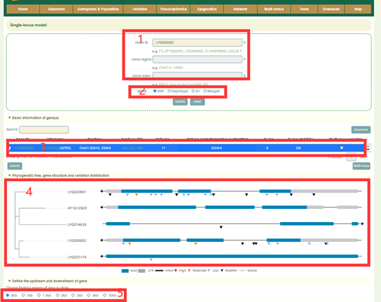
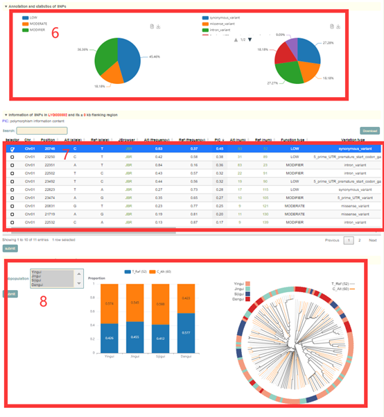
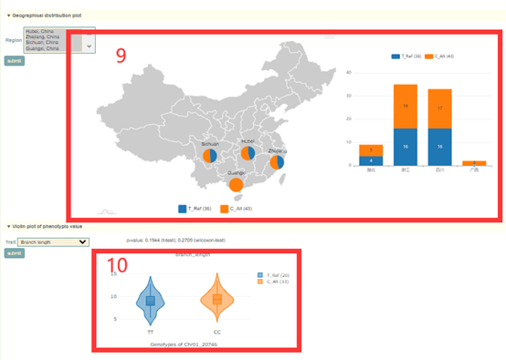
In the Single-locus module, users can search for genetic variation information in genes or genomic regions according to the gene ID, genomic region and gene index (box 1). The database integrated SNPs, InDels and SVs, and users can query by SNP or SV mode (box 2). In addition, users can also analyze the haplotypes composed of multiple SNPs in a gene through Haplotype mode, or perform combined analysis of SNPs and SVs using the merge mode (box 2). Take the search for the LYG000002 gene as an example, the user enters “LYG000002” in the Gene ID, then selects the SNP (box 2), and then clicks 'submit' to query to obtain the related information. The first page of the results is the statistics of the variation data of all homologous genes of the LYG000002 gene in the Liuyejingui genome, such as the number of SNPs and SVs in the gene region (box 3). This is followed by a visualization of the distribution of variants in homologous genes, where different colored triangles represent variants with different variation effects. The user can move the mouse to the position of the corresponding mutation to view the specific information of the mutation (box 4). Then there is the LYG000002 gene structure diagram, the user can move the mouse to the position of the corresponding variant and click to select the specific information to view the variant (box 5). Next, the user will get the statistics of the variants contained in the gene (box 6) and a list of all variants (box 7). The user can check the variant he wants to find in the first column. Then, based on the variant selected by the user, the page will give the frequency distribution of the variant in different subgroups (box 8) and the frequency distribution in the population in different geographic regions (box 9). Then, users can submit the phenotype to browse in the phenotype search bar to view the difference in phenotype values of accessions with different genotypes (box 10).

3.2 Multi-locus module

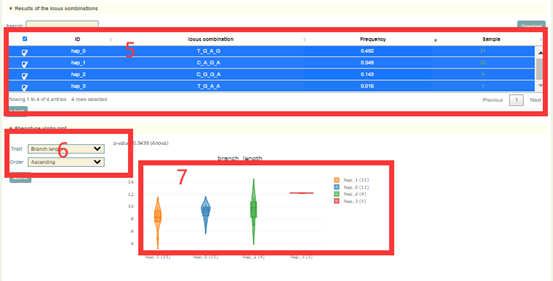
In the Multi-locus module, the user first entered the multiple gene IDs to query in the search box, and clicks 'submit' to submit (box 1). Next, as for the queried genes (box 2), the user selects the SNP ID to query and clicks 'submit' to submit (box 3). Then, the page will list the different haplotypes composed of these SNPs and haplotype frequencies (box 5). After users checked the haplotype they want to query in the first column, the page will list the sequence composition of the haplotype (box 4) based on the variants selected by the user. Then, the page will list the difference in phenotype values corresponding to accessions with different haplotypes(box 6). Users can also submit genes of interest in the gene search bar to view the differences in gene expression levels of accessions with the different haplotypes (box 7).

3.3 About

All resequencing reads of the O. fragrans 161 accessions were mapped to the "Liuyejingui" reference genome ^[1]. SNP calling was performed using the Genome Analysis Toolkit (v4.1.4.1) ^[2]. The SNPs in the joint genotyping were further filtered to remove SNP sites with MAF < 0.05, sequencing depth < 4, and those that had samples with missing data. Finally, 2,022,974 high-quality variants were obtained, including 1,913,050 SNPs and 109,924 InDels. The large indels (> 50bp) in O. fragrans 161 accessions were identified using previous published software IndelEnsembler ^[3]. Totally, 818,412 large indels were obtained, including 322,517 deletions (DELs), 64,194 duplications (DUPs), and 431,701 insertions (INSs). The annotations and effects of SNPs on gene function were predicted using SnpEff (v5.0) software ^[4]. There are 163,725 variants in the gene coding sequences, 342 disruptive inframe InDels, and 2,829 variants caused potentially large effects such as stop codon gain or loss. To explore the effect of variants on O. fragrans phenotypes, we developed the "Variation" module. The "Variation" module integrates genetic variation, and phenotype data, providing descriptions about the effect annotation, phenotype of genetic variations, and genotype-phenotype associations. In this module, users can enter the gene name, gene ID, or chromosome region to screen the candidate variations/genes for certain traits in the Single-locus or Multi-locus model.

References

1. Chen H, Zeng X, Yang J, Cai X, Shi Y, Zheng R, et al. Whole-genome resequencing of Osmanthus fragrans provides insights into flower color evolution. Hortic Res 2021, 8:98.
2. McKenna A, Hanna M, Banks E, Sivachenko A, Cibulskis K, Kernytsky A, et al. The Genome Analysis Toolkit: a MapReduce framework for analyzing next-generation DNA sequencing data. Genome Res 2010, 20:1297-1303.
3. Liu DX, Rajaby R, Wei LL, Zhang L, Yang ZQ, Yang QY, et al. Calling large indels in 1047 Arabidopsis with IndelEnsembler. Nucleic Acids Res 2021, 49:10879-10894.
4. Cingolani P, Platts A, Wang le L, Coon M, Nguyen T, Wang L, et al. A program for annotating and predicting the effects of single nucleotide polymorphisms, SnpEff: SNPs in the genome of Drosophila melanogaster strain w1118; iso-2; iso-3. Fly (Austin) 2012, 6:80-92.

4. Transcriptomics

4.1 Expression profile

Expression profile (Liuyejingui library) module can facilitate the identification of gene functions, which is greatly needed in Osmanthus fragrans.

We collected RNA sequencing data from a total of 11 previous studies, including different tissues, or under different treatment conditions. The tissues mainly come from root, stem, leaf, callus, and various tissues in flowers. Environmental stresses mainly include relatively low temperature stress, ethephon, sodidum thiosulfate and 5'-azacytidine.

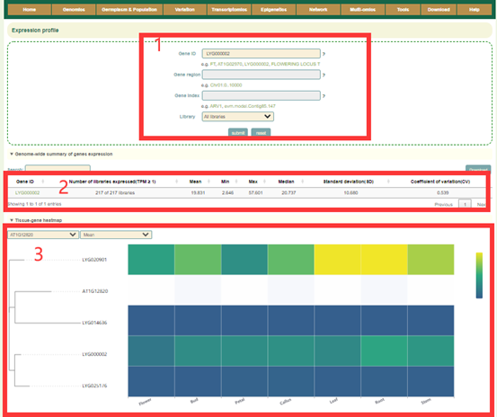
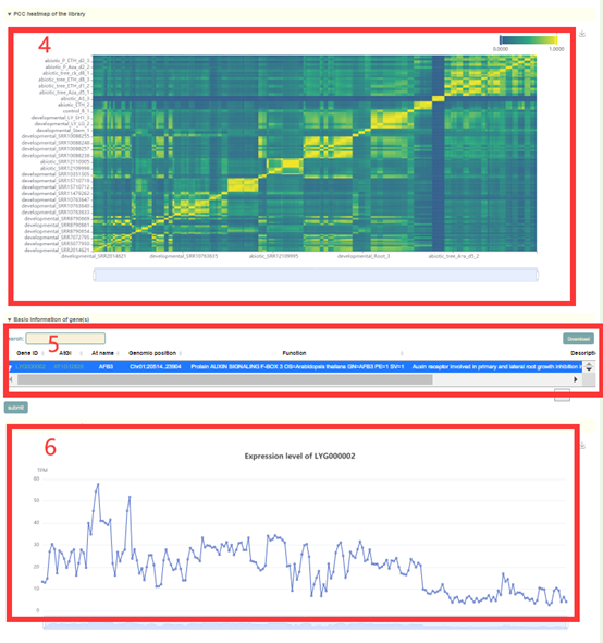
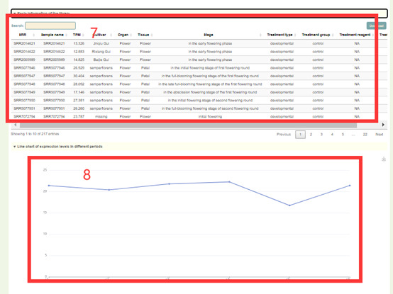
In this module, Users can search the expression level information of the gene of interest through three gene modes including gene ID, genome interval and gene index (box 1). For example, when the user enters LYG000002, the information of the genes on the Liuyejingui genome will be obtained first in the "Genome-wide summary of genes expression", including the statistical information of gene expression level is obtained, including how many libraries it is expressed in, the mean, median, maximum, minimum, standard deviation and coefficient of variation of the expression (box 2). Then, the page will give data and visual displays of the expression levels of these genes in all libraries, such as Tissue-gene heatmap heatmaps (box 3), PCC heatmap of the library (box 4), Gene expression level of the library (box 6) and Line chart of expression levels in different periods (box 8). When the user enters LYG000002, the information of the homologous genes on the Liuyejingui genome will be obtained in the "Basic information of genes", including the gene id of the corresponding Liuyejingui genome, the corresponding Arabidopsis thaliana homologous gene ID and gene name, Physical location and functional descriptive information of genes (box 5). Then, the page will give information of the expression levels of these genes in all samples (box 7).

4.2 About

We collected RNA sequencing data from a total of 11 previous studies, including different tissues, or under different treatment conditions. The tissues mainly come from root, stem, leaf, callus, and various tissues in flowers. Environmental stresses mainly include relatively low temperature stress, ethephon, sodidum thiosulfate and 5'-azacytidine.

The quality of the RNA sequencing reads was examined by FastQC (v0.11.9) (https://www.bioinformatics.babraham.ac.uk/projects/fastqc/). Barcode adaptors and low-quality reads (read quality < 80 for paired-end reads) were removed by Trimmomatic (v0.38) ^[1]. Then, the filtered reads were aligned to the O. fragrans "Liuyejingui" reference genome using Hisat2 (v2.1.0) ^[2] with default parameters. Bam files containing aligned reads were inputted into StringTie (v1.3.3b) ^[3] to measure the expression level of genes. Gene-level raw count data files were generated using featureCounts (v1.6.4) ^[4]. The raw count data were imported into Bioconductor package DESeq2 ^[5] in the R language to identify the differentially expressed genes. Genes had a log2-converted fold change ≥ 1 or ≤ -1 with an FDR (False Discovery Rate) ≤ 0.05 were considered as DEGs.

References

1. Bolger AM, Lohse M, Usadel B. Trimmomatic: a flexible trimmer for Illumina sequence data. Bioinformatics 2014, 30:2114-2120.
2. Kim D, Langmead B, Salzberg SL. HISAT: a fast spliced aligner with low memory requirements. Nat Methods 2015, 12:357-360.
3. Pertea M, Kim D, Pertea GM, Leek JT, Salzberg SL. Transcript-level expression analysis of RNA-seq experiments with HISAT, StringTie and Ballgown. Nat Protoc 2016, 11:1650-1667.
4. Liao Y, Smyth GK, Shi W. featureCounts: an efficient general purpose program for assigning sequence reads to genomic features. Bioinformatics 2014, 30:923-930.
5. Love MI, Huber W, Anders S. Moderated estimation of fold change and dispersion for RNA-seq data with DESeq2. Genome Biol 2014, 15:1-21.

5. Epigenetics

5.1 DNA methylation

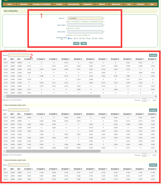
In the DNA methylation module, we integrated data from 18 WGBS-seq libraries and calculated the methylation ratio of each gene region in each library. Users can enter the gene id or genomic region, then set the region size (box1) in Flanking region, and click 'submit' to query. Next, the user will get the information list of the queried genes in box2.

5.2 About

Whole-genome bisulfate sequencing (WGBS) was performed during O. fragrans different stages of flowering: (S1, Linggeng stage; S2, Initial flowering stage; S3, Early full flowering stage; S4, Full flowering stage; S5, Late full flowering stage; S6, Abscission stage). Trimmomatic (v0.38) was used to filter out low-quality reads. The clean reads were then mapped to the O. fragrans "Liuyejingui" reference genome using bitmapperBS software ^[1]. The bisulfite conversion rates were evaluated using lambda DNA. The coverage of cytosine bases across the genome and cytosine-base methylation levels in different contexts were scored using the CGmapTools mstat tool ^[2]. The methylation level was determined by dividing the number of reads covering each mC by the total number of reads covering that cytosine, which was also equal to the mC:C ratio at each reference cytosine.

References

1. Cheng, H. Y. & Xu, Y. BitMapperBS: a fast and accurate read aligner for whole-genome bisulfite sequencing. BioRxiv. 442798 (2018).
2. Guo W, Zhu P, Pellegrini M, Zhang MQ, Wang X, Ni Z. CGmapTools improves the precision of heterozygous SNV calls and supports allele-specific methylation detection and visualization in bisulfite-sequencing data. Bioinformatics 2018, 34:381-387.

6. Network

6.1 Co-expression

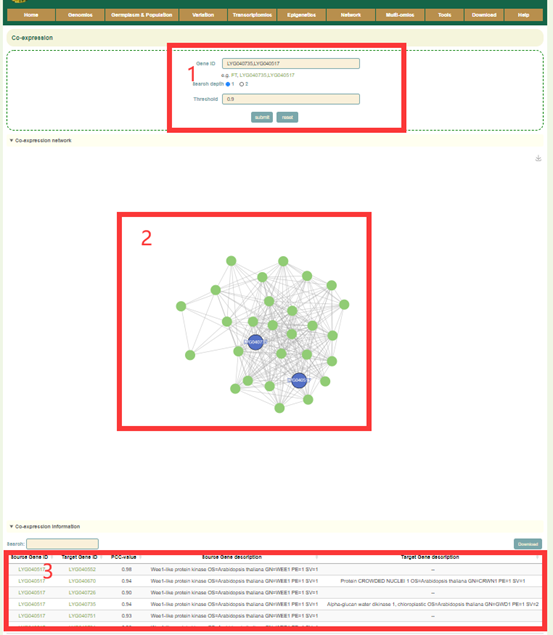
In the Co-expression module, the user first submits one or more gene IDs in the search box, and sets the depth of the network connection (1 or 2) (box1), and then clicks “submit” to submit. Next, the user will obtain the co-expression network figure of the gene or genes (box2) and the pearson correlation coefficients and functional information of the gene or genes (box3).

6.2 TF regulation network

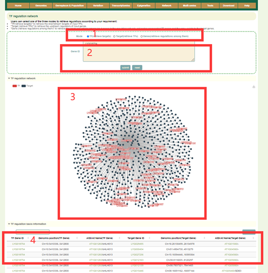
In the TF regulation network module, the user first submits one or more gene IDs (box1) in the search box, and sets the search modes including TF (to retrieve downstream regulated genes), Target (to retrieve the TF genes) or Genes (to retrieve the TF genes and regulated downstream genes) (box2), and then clicks “submit” to submit. Next, the user will get the network figure of TFs and the target genes (box3), the pearson correlation coefficients between them and the function information of the genes (box4).

6.3 About

The data used by the "co-expression" network is the same as that used in the "Expression profile" page. The co-expression network was obtained by calculating the Pearson correlation coefficient (r2) of the gene pairs side by side, and the final gene pairs r2 > 0.8 were retained. Finally, we obtained 17,013,938 co-expressed gene pairs involving 33,654 genes. In addition, combined with the TF annotations, we obtained 1,626 TFs and 36,222 regulated genes, and obtained 2,036,569 TF-gene pairs.

7. Multi-omics

7.1 GWAS

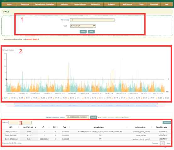
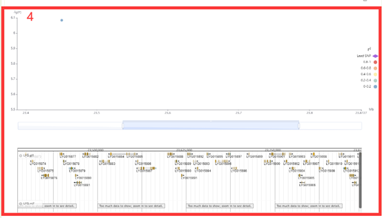
In GWAS module, the user firstly clicked the phenotype name(box1), and then a dialog box for the phenotype list will pop up. The user selects the threshold by checking the first column and then selects phenotype (box1), that is GWAS results for this phenotype can be viewed. The first is a manhattan plot (box2), in which we denote the p-value of each window by the p-value of the most significant SNP in it. Here, the user can zoom in or out by sliding the mouse wheel, and then move the mouse to the corresponding window to browse the lead SNP and the corresponding p-value (box 2) in the window. The user can then click on the bars of this window to view all the significant SNPs within this region along with the corresponding GWAS statistics (box 3) and Manhattan plots (box 4).

7.2 About

Genome-wide association study (GWAS) is an approach for identifying the genes that underlie common diseases and related quantitative traits. This strategy combines a comprehensive and unbiased survey of the genome with the power to detect common alleles with modest phenotypic effects. We collected 4 traits of 161 O. fragrans accessions, including branch length, corolla diameter, flower color, and flower number and performed GWAS combining their genotypes using GEMMA. The most significant SNP in every 500kb-window was retained. User can browse GWAS results and search significant SNPs and genes of 4 O. fragrans traits.

8. Tools

8.1 JBrowser

Moving

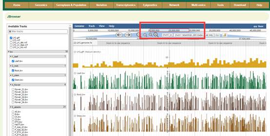
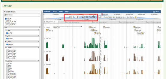
Move the view by clicking and dragging in the track area, or by clicking or in the navigation bar, or by pressing the left and right arrow keys. Center the view at a point by clicking on either the track scale bar or overview bar, or by shift-clicking in the track area.

Zooming

Zoom in and out by clicking or in the navigation bar, or by pressing the up and down arrow keys while holding down "shift". Select a region and zoom to it ("rubber-band" zoom) by clicking and dragging in the overview or track scale bar, or shift-clicking and dragging in the track area.

Showing Tracks

Turn a track on by dragging its track label from the "Available Tracks" area into the genome area, or double-clicking it. Turn a track off by dragging its track label from the genome area back into the "Available Tracks" area.

Searching

Jump to a feature or reference sequence by typing its name in the location box and pressing Enter. Jump to a specific region by typing the region into the location box as: ref:start..end.

Example Searches

"uc0031k.2": searches for the feature named uc0031k.2

"chr4": jumps to chromosome 4

"chr4:79,500,000..80,000,000": jumps the region on chromosome 4 between 79.5Mb and 80Mb

"5678": centers the display at base 5,678 on the current sequence

8.2 Blast

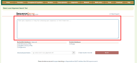
Paste the sequence to be queried in the sequence box below;Select the database type and click 'Submit' to submit.

Results:

The first is a graphical representation of the genomic positions to which the sequences are aligned. Then there is a list of all the positions aligned, and the user can click them to query the detailed sequence alignment.

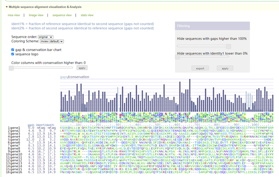
8.3 Multi Alignment Viewer

Enter gene gene list or sequence file; then raw output of result, including visualization of sequences.

8.4 Sequence fetch

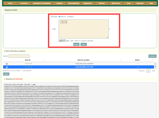
Usage: Paste the gene list to be aligned in the sequence box or upload the gene list file to be extracted and click "Submit" to submit.

Results: You can directly copy the sequences extracted from the dialog box or click on "CDS", "gDNA" and "Protein" in "Download Sequences of all Input Genes" to download these sequences.

8.5 GO enrichment

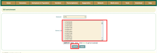
Usage:

Paste the gene list in the sequence box or upload the gene list file, and click Submit.

Results:

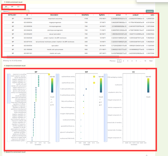
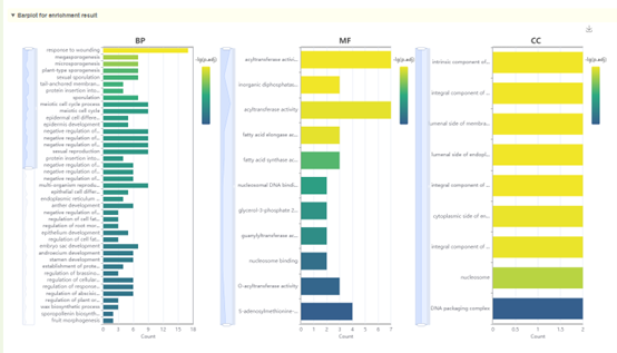
1. List of results of GO enrichment analysis. You can switch the category of GO by clicking BP, MF and CC above, and click "Download" in the upper right to download;

2. The dot plot and bar plot of GO enrichment analysis results. Move the mouse over the figure to query the statistics of the corresponding GO enrichment analysis results. Click the arrow at the top right to download the image.

8.6 KEGG enrichment

Usage:

Paste the gene list in the sequence box or upload the gene list file, and click "Submit" to submit;

Results:

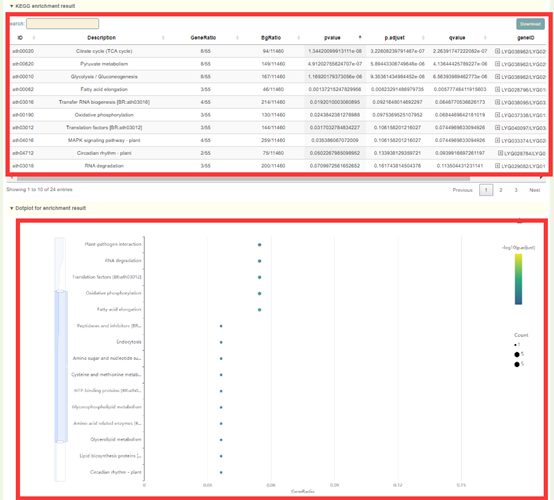
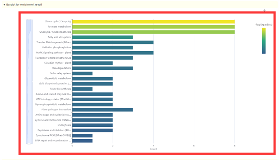
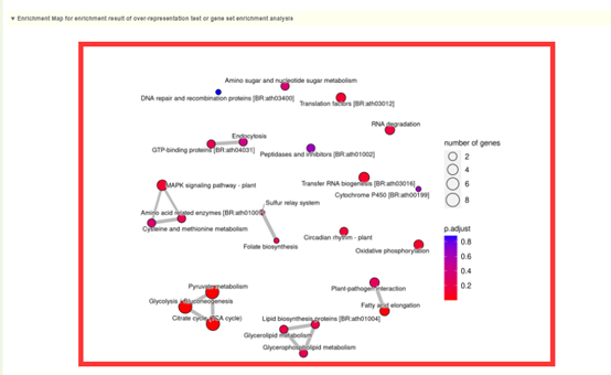
1. The result list of KEGG enrichment analysis. Click “Download” in the upper right to download;

2. Dot plot, bar plot and network plot of KEGG enrichment analysis results. Move the mouse over the figure to query the statistics of the corresponding KEGG enrichment analysis results. Click the arrow at the top right to download the image.

8.7 SNP match

Usage:

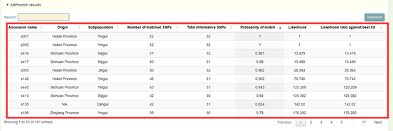
Paste the genotype data (VCF format) of the sample to be identified in the sequence box or upload the genotype file (VCF format) of the sample and click Submit. SNPmatch will then predict the similarity between the accession to be queried and the 2311 accessions based on the genotype information and output the accessions with a similarity of larger than 0.5.

Results:

1. The result list of SNPmatch: Click "Download" at the top right to download;

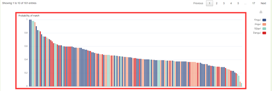
2. The bar plot of SNPmatch results, the x axis is the accession name in the population similar to the input accession, and the y axis is the similarity with the sample. Move the mouse to the figure to query the corresponding data. Click the arrow at the top right to download the image.

8.8 Primer3

Usage:

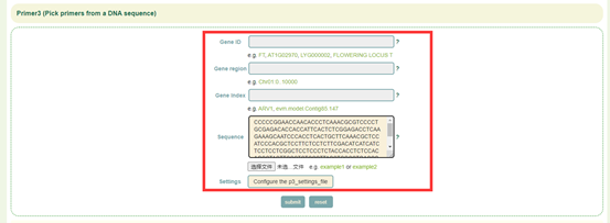
1. Enter gene ID, genomic region, gene index, or upload gene list or sequence file;

2. Click “Configure the p3_settings_file” to change the parameters of the configuration file or upload the configuration file;

3.Select the genes to be designed in primers and submit.

Results:

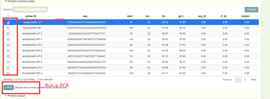
1. The statistical results of primer design: Click “Download” in the upper right to download. Users can select primers for e-PCR alignment;

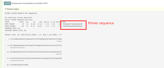
2. Raw output of Primer3, including visualization of primer sequences and their positions on the genome.

8.9 e-PCR

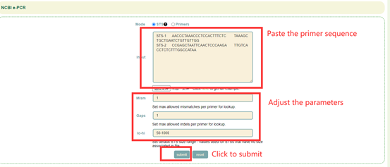
Usage:

1. Select the file format (STS or Primers) in Mode;

2. Paste the sequence into the dialog or upload the sequence file;

3. Adjust alignment parameters, including mismatch value(mism), gap size(gap) and sequence length range(lo-hi);

Click Submit.

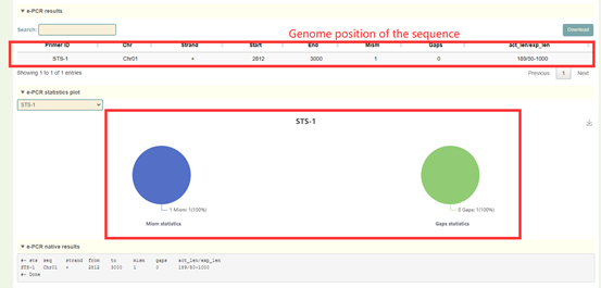
Results:

1. The list of e-PCR results, each row is the position of the sequence amplified by the primers;

2. Statistical chart of e-PCR comparison results, including the ratio of mismatches and gaps;

3. The raw output result of e-PCR.