AMIR: Asteraceae multi-omics information resource

Tutorial

1. Species (Tutorial video)

The following tutorial video will provide a comprehensive overview of this module.

Alternatively, users can explore the tutorial below to learn about the functionality of this module.

1.1 Species

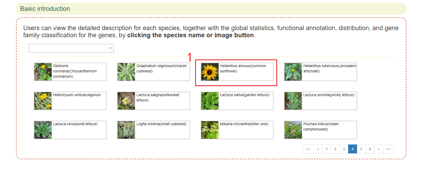
Species module provides an overview of the species that were analyzed, obtained from 74 species of Asteraceae family. In this module, users can query the basic information of 74 plants, as well as Pfam and gene family information for 54 species with available annotated files.

In this page, users can enter scientific name or common name of the species of interest to get the related information. For example, if users enter 'Helianthus annuus' in box 1, results in boxes 2 to 8 will be obtained.

Firstly, box 2 provides an overview of the entered species, including species introduction and all collected version information for the species. Genomic information with annotated files is listed separately in box 3.

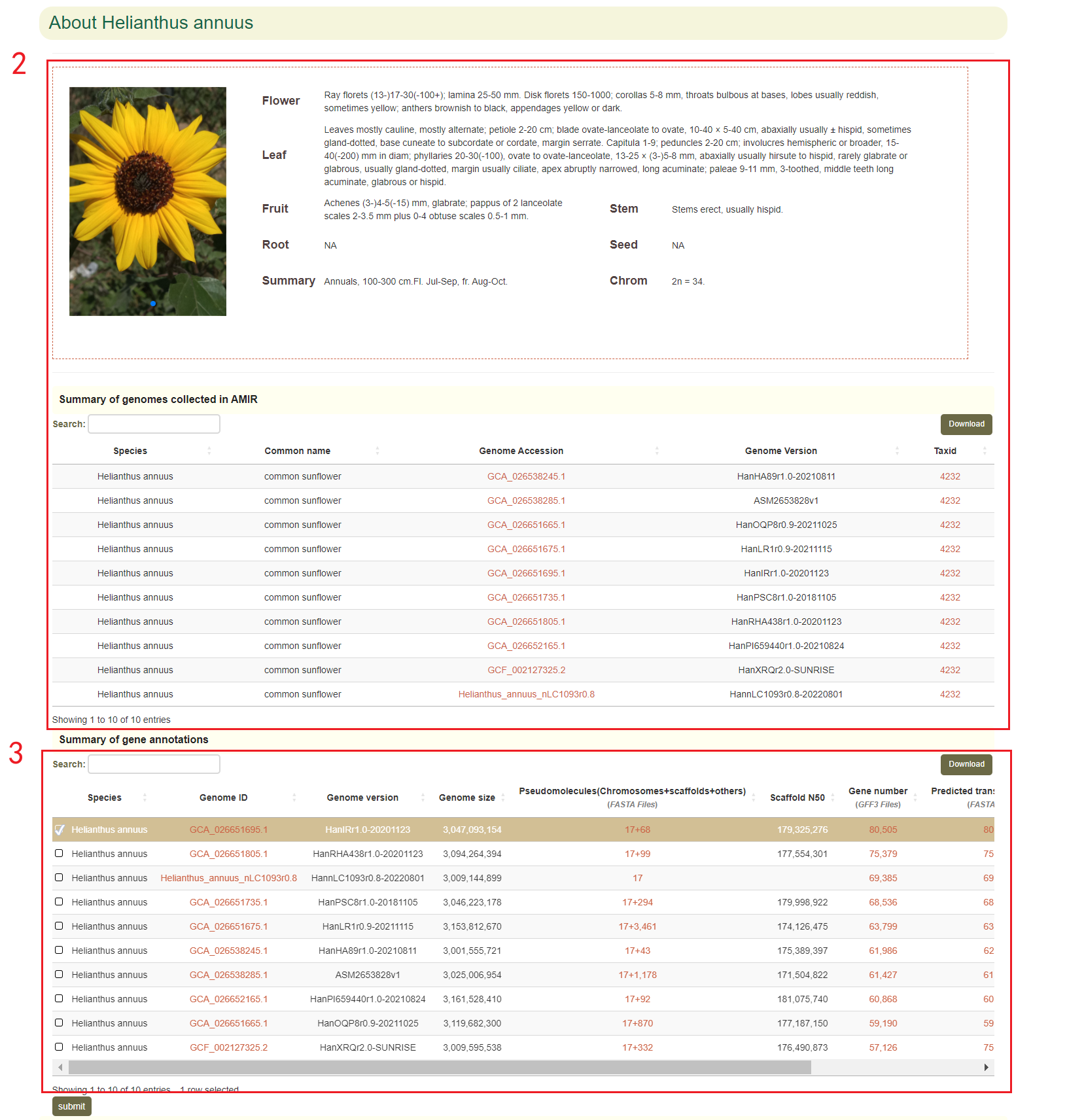
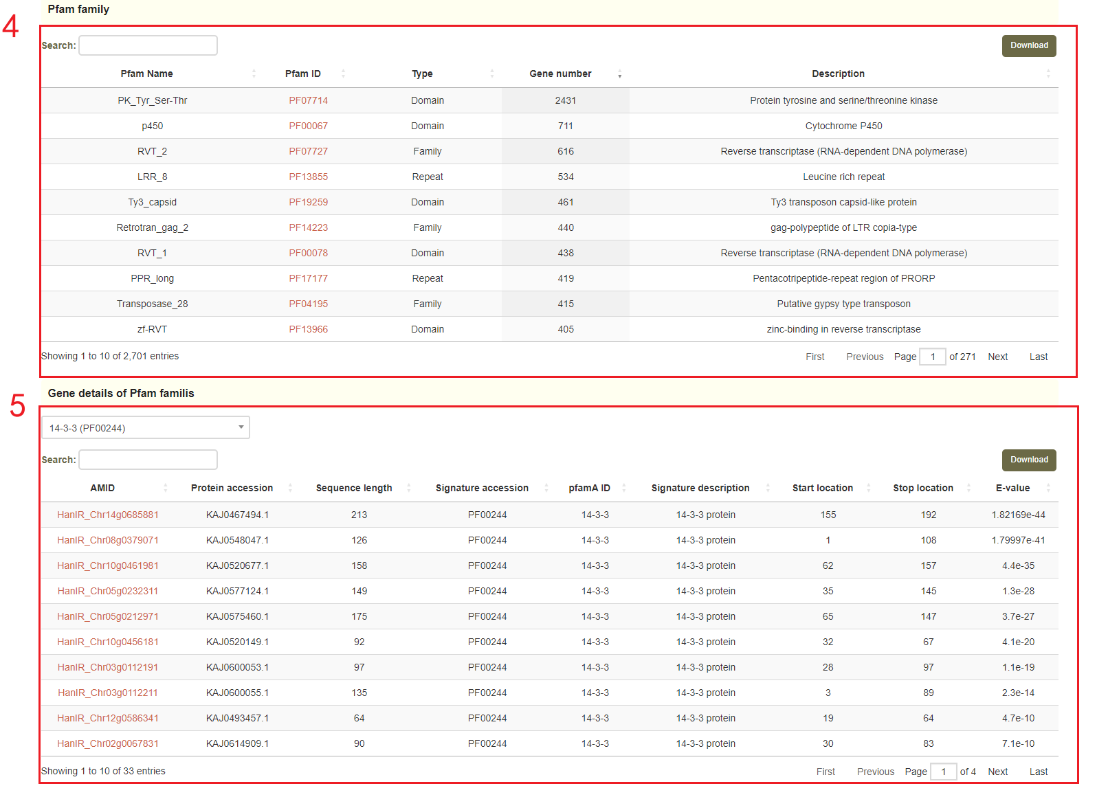
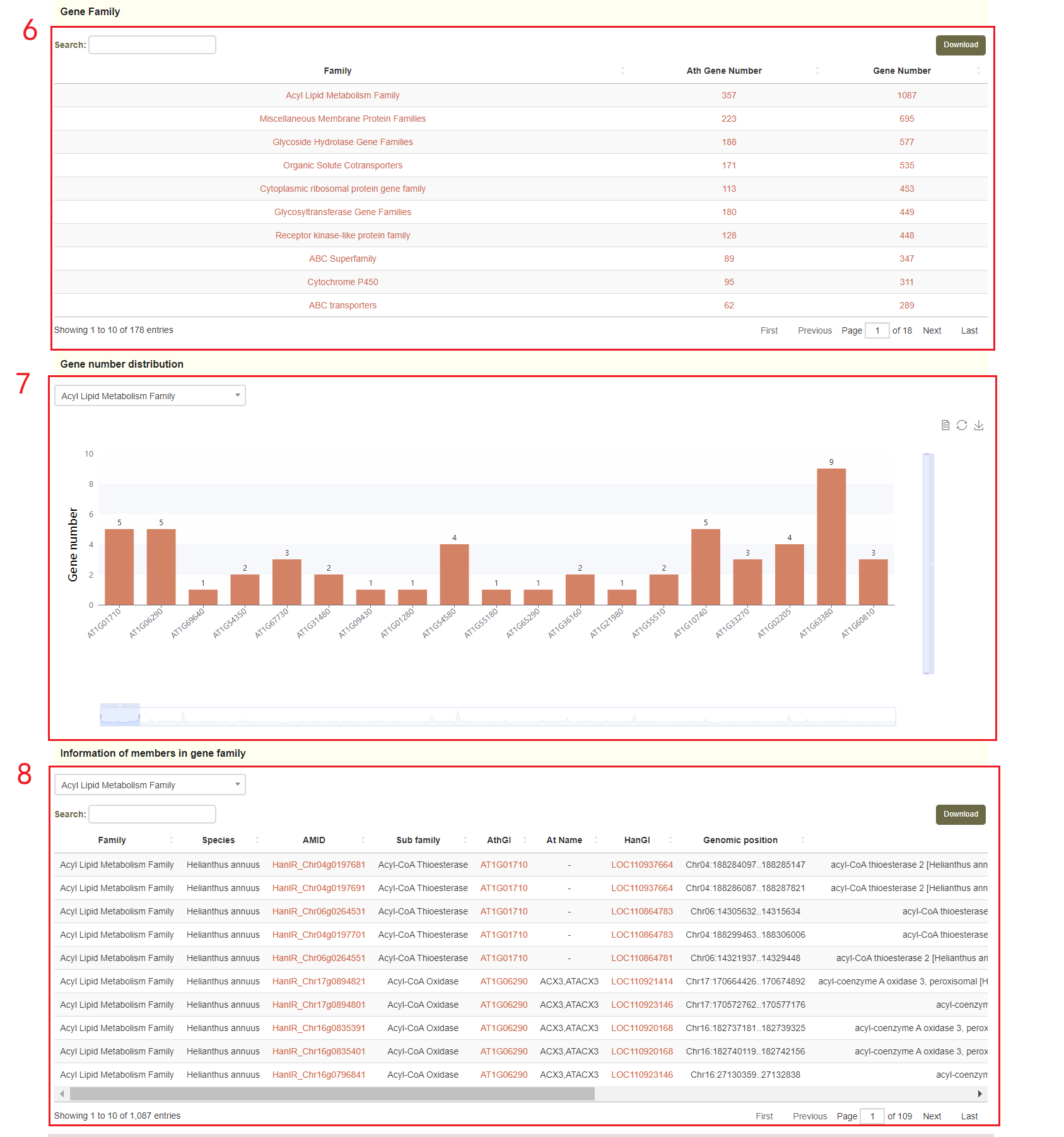
Next, users will obtain genes protein classes(box 4 and box 5) and gene families(boxes 6-8), based on the selected annotated version.

1.2 About

The Species module provides overview of Asteraceae. In this module, users can access basic information for 74 species, as well as Pfam and gene family information for 54 species with available annotated files.

1.3 References

Weakley, A.S., and Southeastern Flora Team. 2024. Flora of the southeastern United States Web App. University of North Carolina Herbarium, North Carolina Botanical Garden, Chapel Hill, U.S.A. fsus.ncbg.unc.edu Accessed Jun 23, 2024.

2. Genomics (Tutorial video)

The following tutorial video will provide a comprehensive overview of this module.

Alternatively, users can explore the tutorial below to learn about the functionality of this module.

2.1 Genome

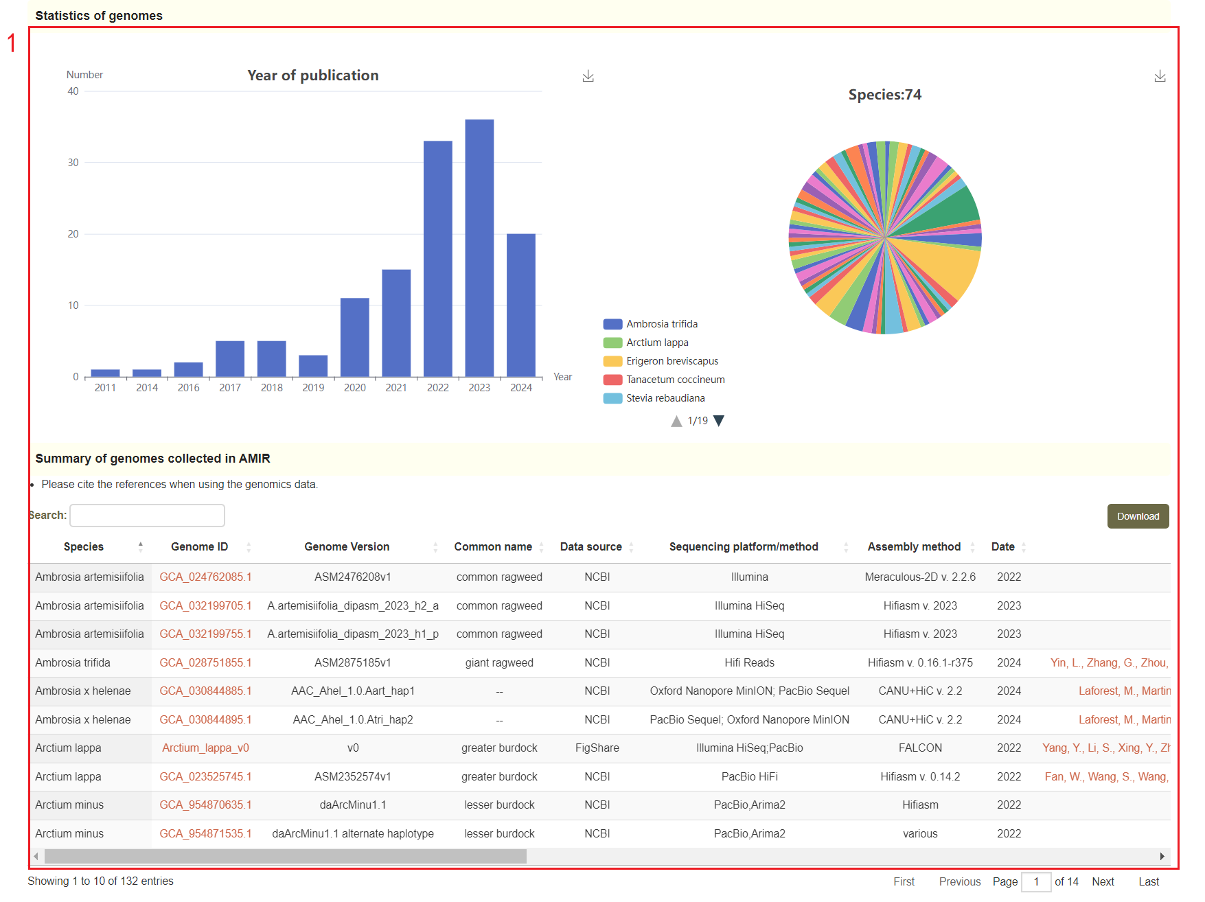
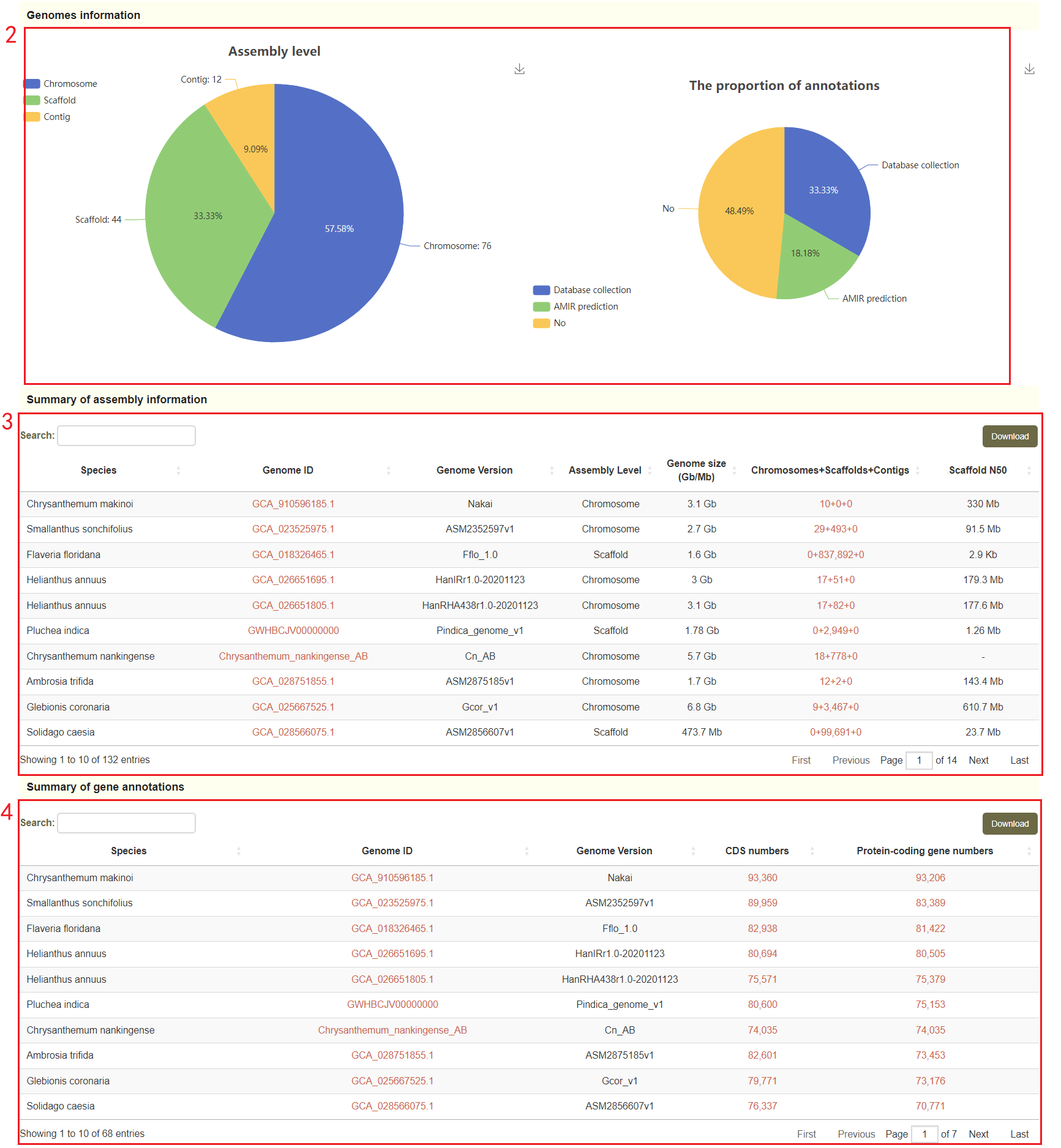
In the genome data page, users can access the data source information of the genome, as well as the visualization of these genomes publication years and distribution in species of Asteraceae family(box 1). The annotation information of the genome is also visualized(box 2), and the user can click on the red number to download the genome file and annotation file(box 3 and box 4).

2.2 Gene search

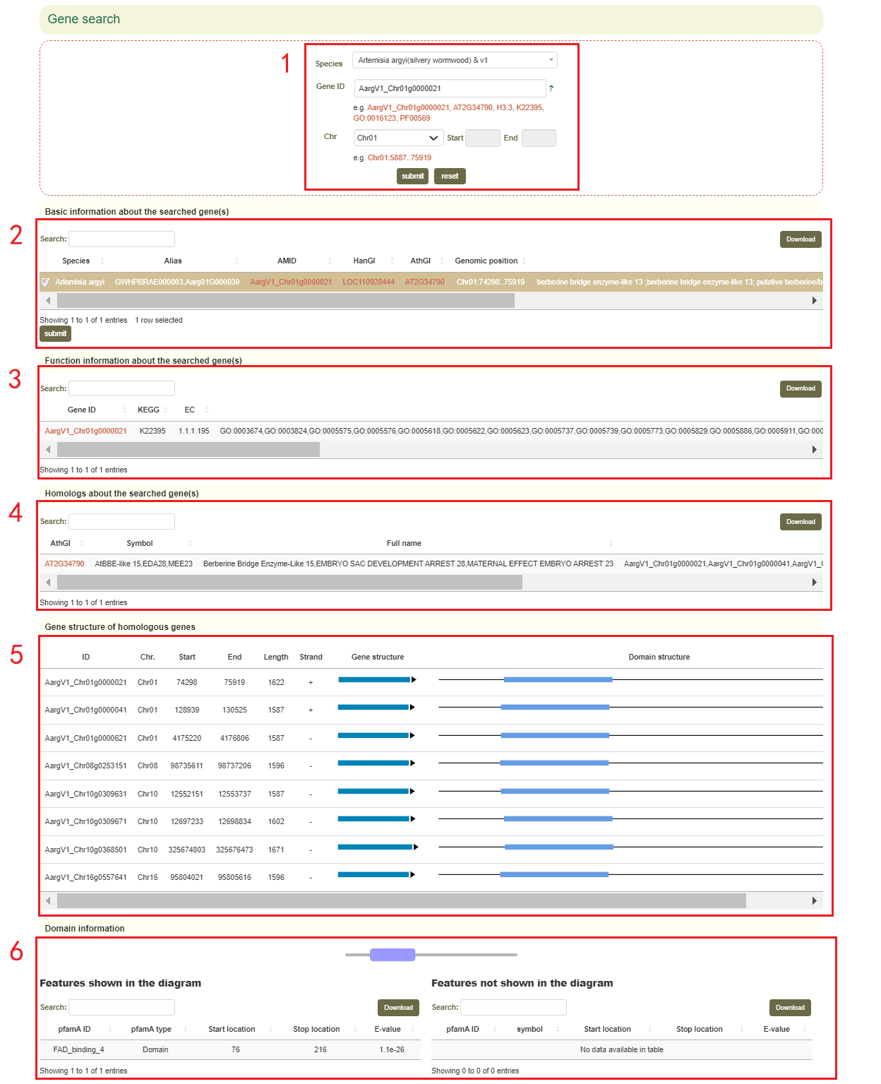
The Gene search page provides gene structure and function information for 68 genomes from 54 species within the Asteraceae family. In this module, the user can enter the gene ID, GO/KEGG/Pfam identifiers to query the related information of the interesting gene. If users entered the gene ID or gene name of Arabidopsis thaliana, the structure and function information of all homologous genes can be obtained.

For example, if users enter 'AargV1_Chr01g0000021' (box 1), they can obtain the physical location and functional description of all homologous genes corresponding to this gene (box 2, box 3 and box 4), as well as the structure of these homologous genes (box 5), and the domain visualization of this gene (box 6)

2.3.1 Gene family information

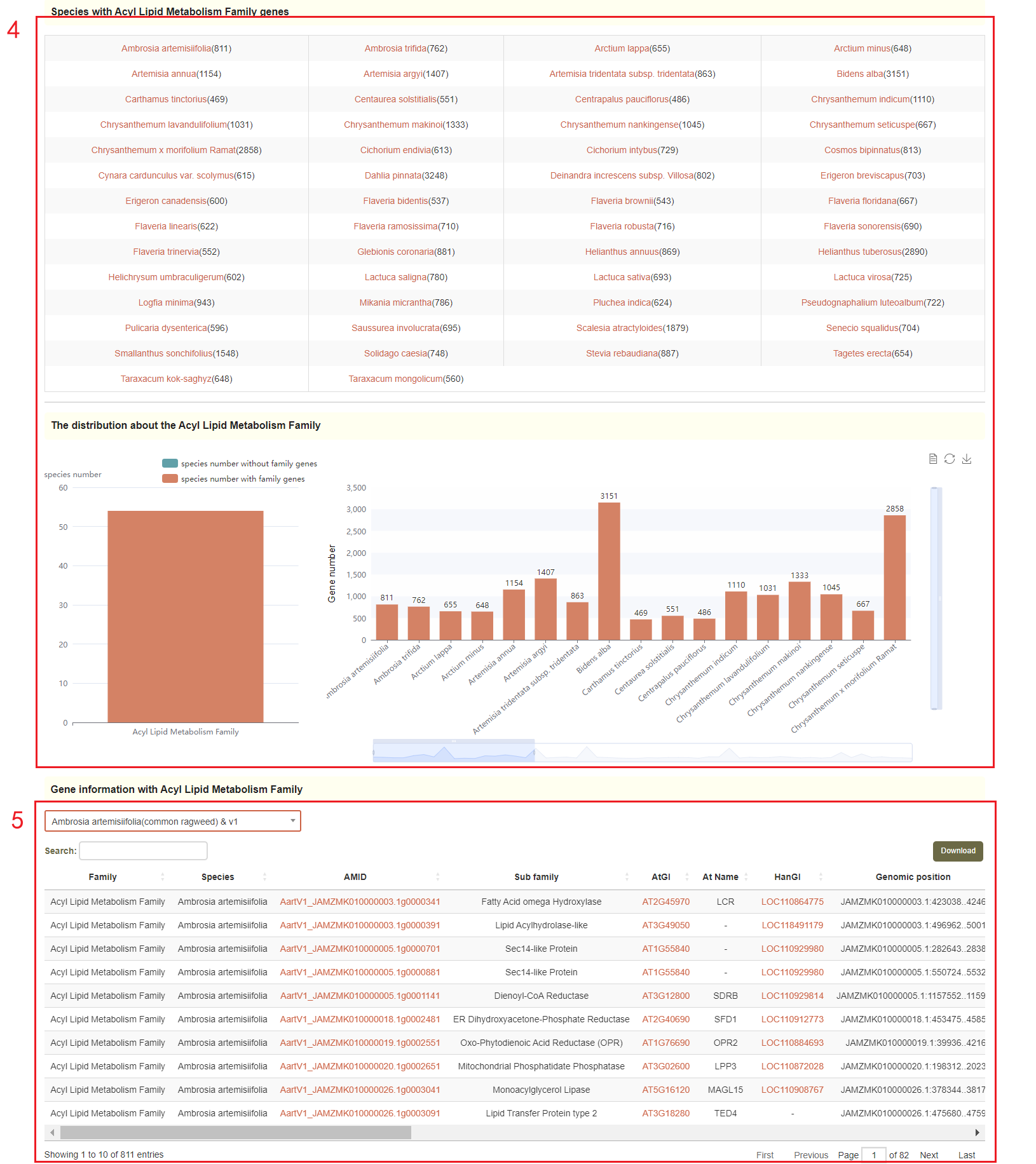
Gene family module integrates information from 181 gene families. The species number and gene number of each gene family are listed in the Gene family overview(box 1), and the visualization of statistics for 181 gene family will be presented(box2). Users can click on the family or enter the family of interest to query the distribution of gene numbers(box 3) and gene number of your selected gene family in each species(box4), as well as gene details of your selected gene family and species(box 5).

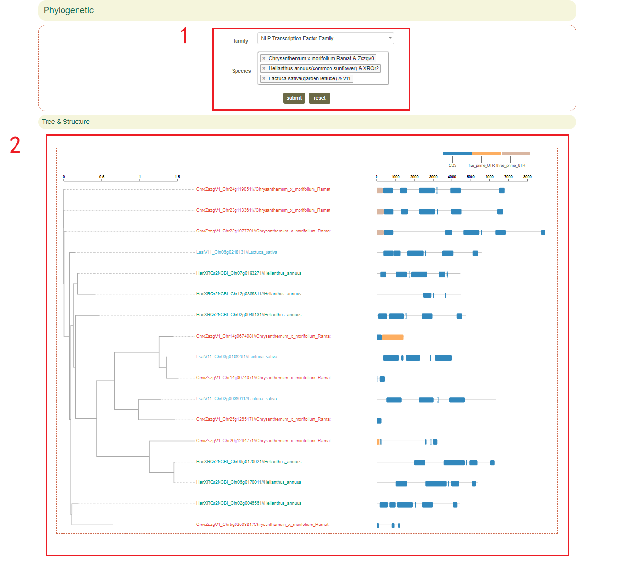
2.3.2 Phylogenetic

The Phylogenetics module provides a cross-species comparison of phylogenetic relationships based on gene families. In this page, users can enter the gene family and species of interest(box 1), then a complete view of orthologs and paralogs of genes in the gene family can be accessed(box 2).

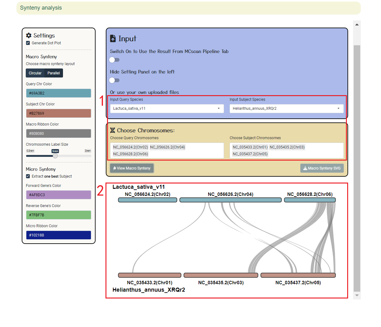
2.4 Genome synteny

Users can browse the alignment results of all regions between genomes using ShinySyn. In ShinySyn the user selects the gene alignment object to view (box 1) and then retrieves the result (boxes 2-4).

2.5 Transcription factor(TF)

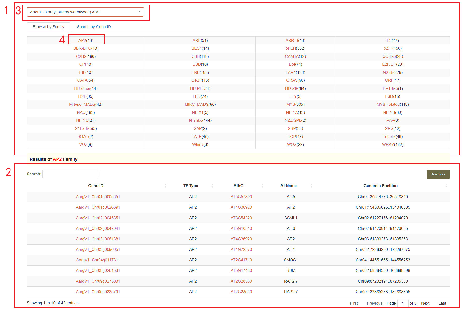
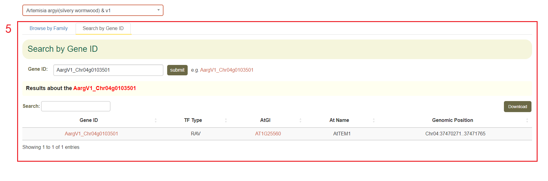
In the transcription factor module, we annotated the genes transcription factor families using PlantTFDB ^[1] and iTAK ^[2].

Users can browse the number of genes in all gene families by using "Browse by Family" (box 1). They can then select the Asteraceae genome in box 3 and view the number of genes in a specific family by clicking on the gene family name. For example, if you select the Artemisia argyi v1 genome (box 3) and click on AP2 (box 4), you will be presented with a list of genes belonging to the AP2 family (box 2).

Additionally, users can also enter a gene ID in the "Search by Gene ID" option to check whether the gene is a transcription factor and obtain its gene family information(box 5).

2.6 Pan-genome

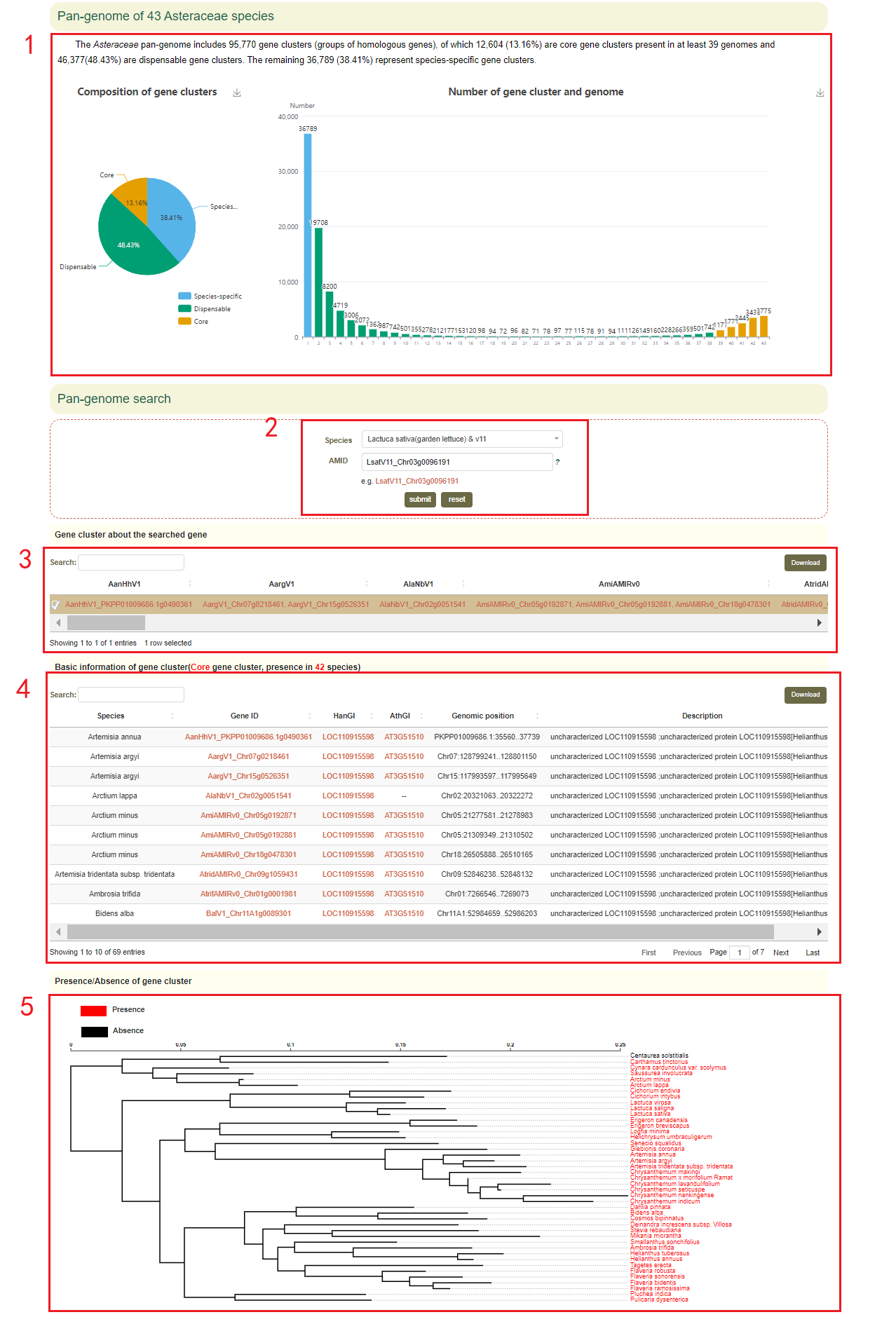
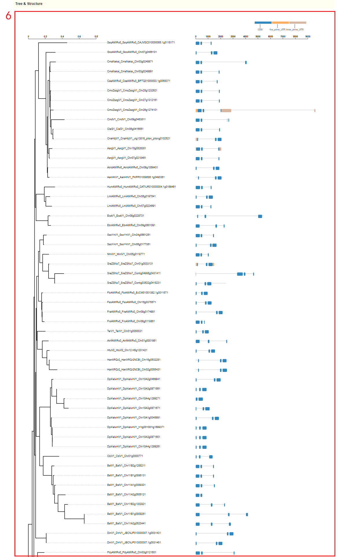
In Pan-genome module, first the user can obtain an overview of the Asteraceae pan-genome, including a visual presentation of the amount of core, dispensable, species-specific in Pan-genome(box 1). Then users can enter the species and genes of interest to obtain the gene cluster and physical location and functional description information of these genes(boxes 2-4). The presence/absence of the gene cluster is also visualized(box 5). Then a complete view of orthologs and paralogs of genes in the gene cluster can be accessed(box 6).

2.7 Homolog search

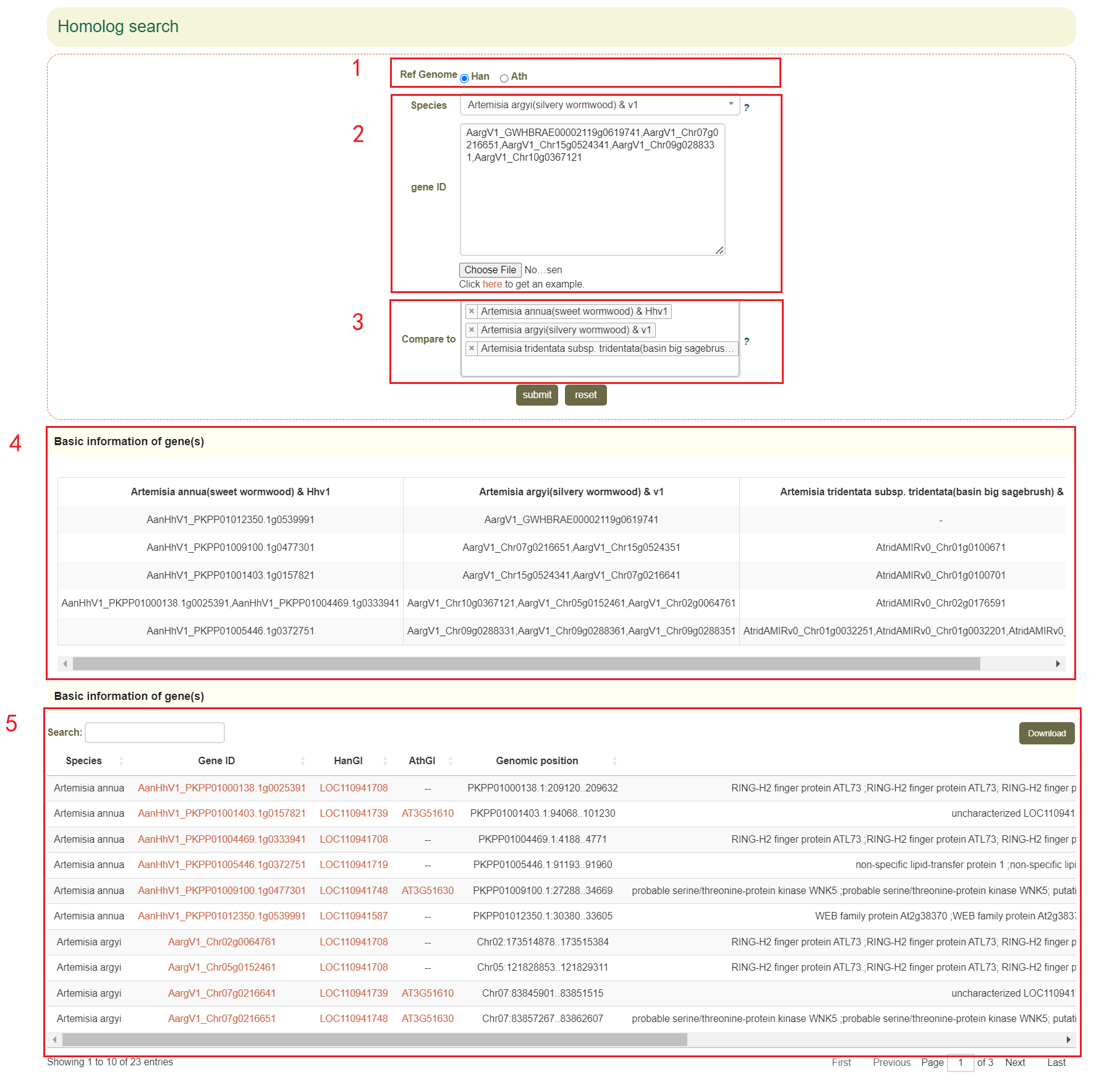
The Homolog search page provides homologous genes query results for 68 genomes within the Asteraceae family. Firstly, users can choose to search for orthologous genes based on Arabidopsis or Sunflower(box 1), then users can select the genome of interest and enter some gene IDs (box 2). Finally, users can select other genomes of interest to identify homologs and paralogs in the selected genomes(box 3 and box 4), as well as obtain the physical location and functional description of all homologous genes(box 5).

2.8 Genome variations

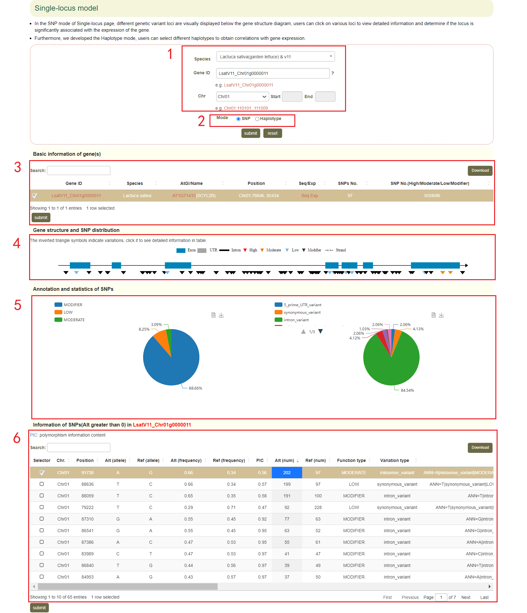
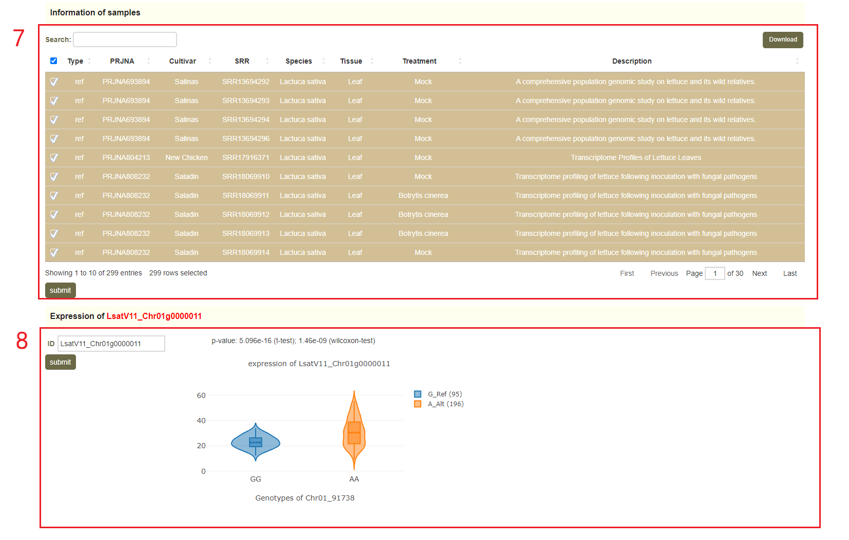
In the Genome variations page, users can search for genetic variation information according to the gene ID or genomic region(box 1). Users can query by SNP or Haplotype mode (box 2). In Haplotype mode, users can analyze the haplotypes composed of multiple SNPs in a gene. Take the search for the LsatV11_Chr01g0000011 gene as an example, users enter “LsatV11_Chr01g0000011” in the Gene ID, next selects the SNP (box 2), and finally clicks 'submit' to query for the related information. The first page of the results is the statistics of the variation data for the LsatV11_Chr01g0000011, such as the number of SNPs in the gene region (box 3). This is followed by a visualization of the distribution of variants in homologous genes, where different colored triangles represent variants with different variation effects. The user can move the mouse to the position of the corresponding mutation to view the specific information of the mutation (box 4). Next, the user will get the statistics of the variants contained in the gene (box 5) and a list of all variants (box 6). Users can also obtain all sample information for reference and alternative alleles(box 7), and violin plots of the expression levels of "LsatV11_Chr01g0000011" in these samples(box 8).

2.9 About

We collected 132 genomes from 74 species within the Asteraceae family and 4,408,432 genes have been annotated (see “Genome” module). We provide gene annotations from seven different perspectives, including homology with Arabidopsis and sunflower, gene and transcription factor families (PlantTFDB ^[1] and iTAK ^[2]), gene ontology ^[3], KEGG pathway (https://www.genome.jp/kegg/) and Pfam domains ^[4] (Table 1). Users can quickly retrieve 11,475,543 annotation data for individual genes or gene sets by searching with gene IDs, GO/KEGG/Pfam identifiers, or transcription factor/gene family names. The synteny analysis was carried out using MCScanX ^[5], and users can use genome synteny module to browse the alignment results between genomes. We have established the first pan-genome for the Asteraceae family based on OrthoFinder ^[6]. This pan-genome includes 95,770 gene clusters (groups of homologous genes).

We used the Braker3 ^[7] to perform gene structure annotation on 24 Asteraceae genomes with high assembly quality but lacking gene annotations. Braker3 integrates three annotation methods, including ab initio gene prediction, homology protein-based gene prediction and RNA-seq based gene prediction. The homology protein library includes protein sequences from Arabidopsis, sunflower, cultivated Chrysanthemum, and lettuce, while the transcriptome data used samples from various tissues and treatments with a mapping rate greater than 80%.

Variations, including 30,507,963 SNPs and 12,257,327 InDels, have been identified based on the transcriptomes. To explore the effect of variantions on gene expression, we developed the "Variation" page. The "Genome variations" page integrates genetic variation, and gene expression data, providing descriptions about the effect annotation, and genotype-gene expression associations. In this page, users can enter the gene name, gene ID, or chromosome region to screen the candidate variations that correlate with gene expression in the Single-locus or Multi-locus model.

SNP calling was performed using the Genome Analysis Toolkit (v4.1.4.1) ^[8]. The SNPs in the joint genotyping were further filtered to remove SNP sites with MAF < 0.05, and those that had samples with missing data. The annotations and effects of SNPs on gene function were predicted using SnpEff (v5.0) software ^[9].

2.10 References

3. Transcriptomics (Tutorial video)

The following tutorial video will provide a comprehensive overview of this module.

Alternatively, users can explore the tutorial below to learn about the functionality of this module.

3.1 Single Species Gene Expression Profile

Gene expression profile module can facilitate the identification of gene functions, which is greatly needed in Asteraceae species. Gene expression profile module contains gene expression levels from 3,897 libraries of 44 species within the Asteraceae family.

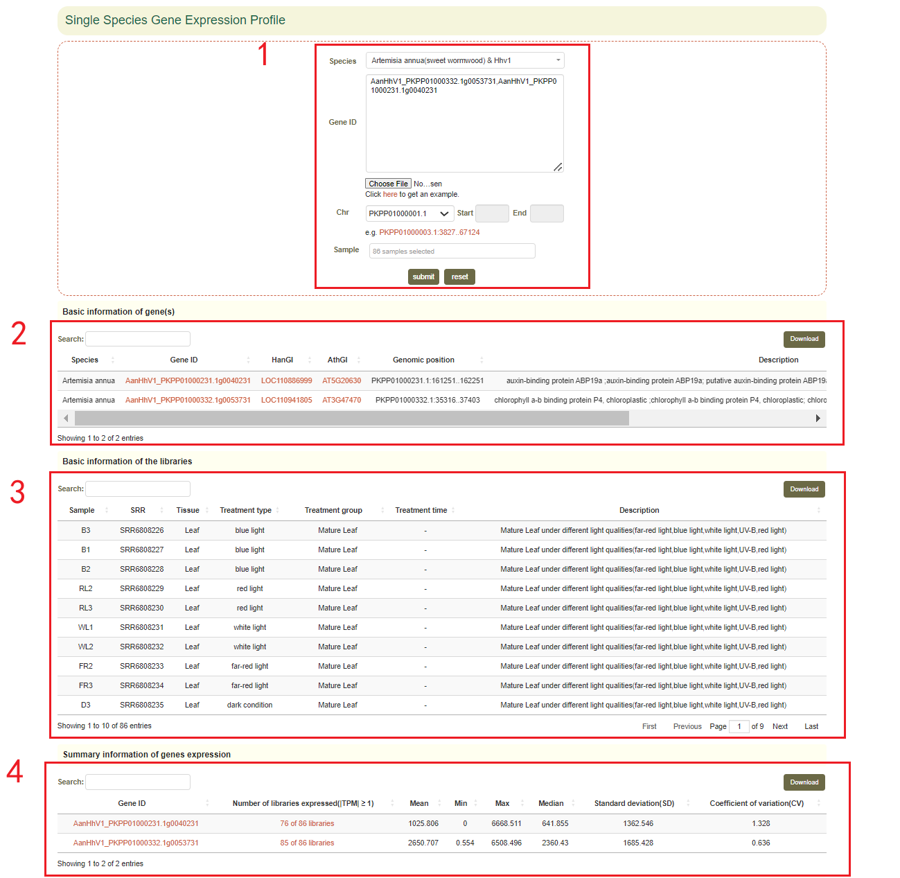
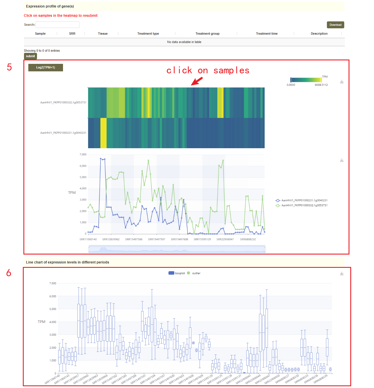
In this module, users can search the expression level information of the gene of interest through two gene modes including gene ID and genome region(box 1). For example, when the user enters some genes of interest(box 1), the information of these genes will be obtained in the "Basic information of genes", including the corresponding Arabidopsis thaliana homologous gene ID, corresponding Helianthus annuus homologous gene ID,the physical location and functional descriptive information of genes (box 2). Then, in box 4, the statistical information of gene expression level is obtained, including how many libraries it is expressed in, the mean, median, maximum, minimum, standard deviation and coefficient of variation of the expression. Finally, the page will give data and visual displays of the expression levels of these genes in all libraries, such as heatmaps (box 5), line graphs (box 5), and boxplots (box 6). Users can also click on samples in the heatmap to resubmit(box 5).

3.2 Mutil Species Gene Expression Profile

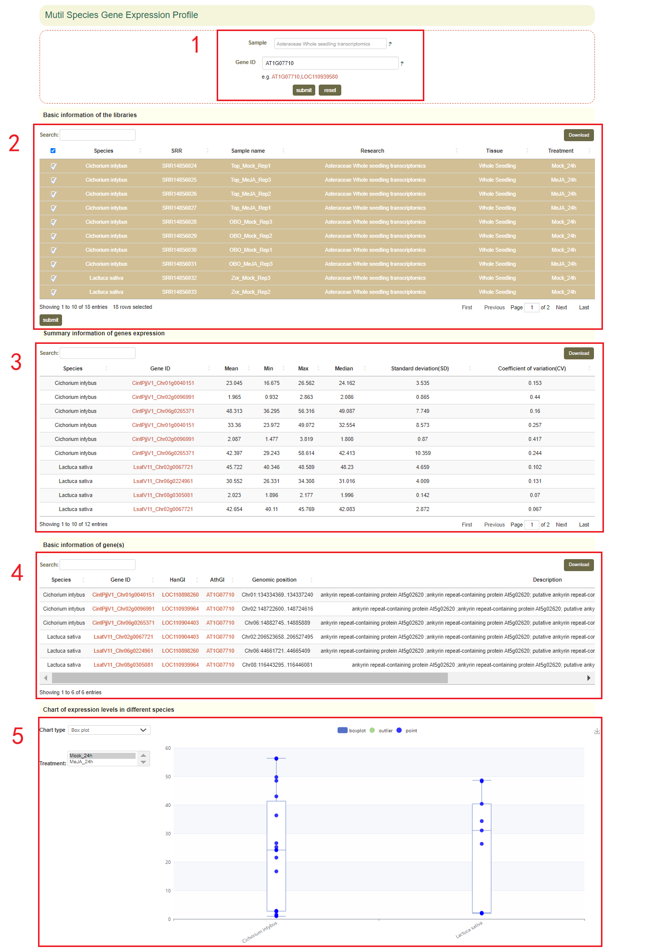
In this page, users can select different datasets and input the gene ID or gene name of Arabidopsis to obtain the expression levels in different species and treatment groups of all orthologs corresponding to that gene. For example, if users entered 'AT1G07710' (box 1), users can obtain the basic information of the dataset that they selected(box 2), the physical location and functional description information of all the orthologous genes corresponding to the gene(box 4), and the statistical information on the expression levels of the orthologous genes(box 3). Then, the page will use boxplots to visualize data showing the expression levels of these genes from different species.

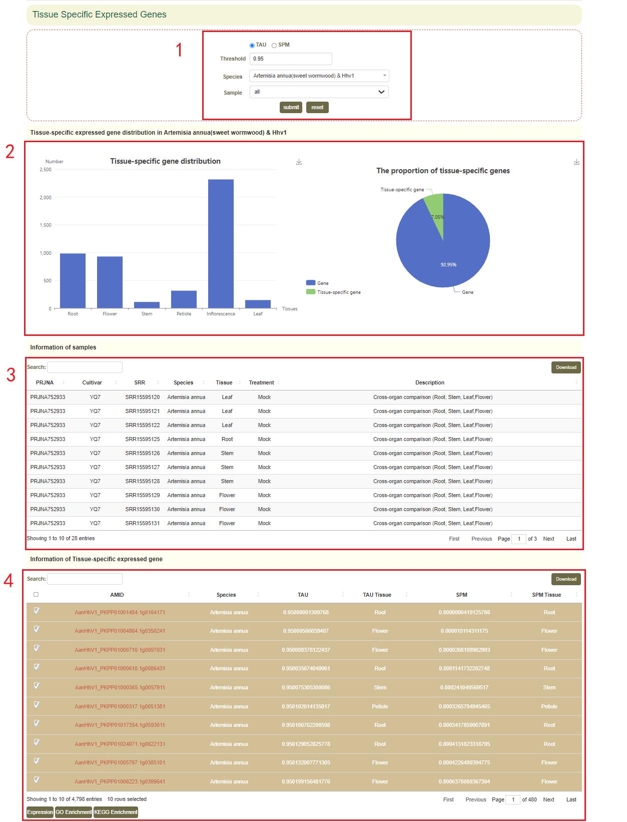
3.3 Tissue-specific Expressed Genes

The “Tissue-specific (TS) expressed genes” page can help you find tissue/sub-tissue-specific genes in the species of interest.

In “Tissue-specific (TS) expressed genes” module, users can choose Tau or SPM and adjust appropriate thresholds to query the tissue-specific expressed genes in the tissue development RNA-seq libraries. Then the page will show the distribution of tissue-specific expressed genes in different tissues and the proportion of all genes in the genome of the species(box 2). Users can obtain the information of samples(box 3). Users can also click on the GO Enrichment or KEGG Enrichment to perform an enrichment analysis of the top 10 tissue-specific expressed genes(box 4).

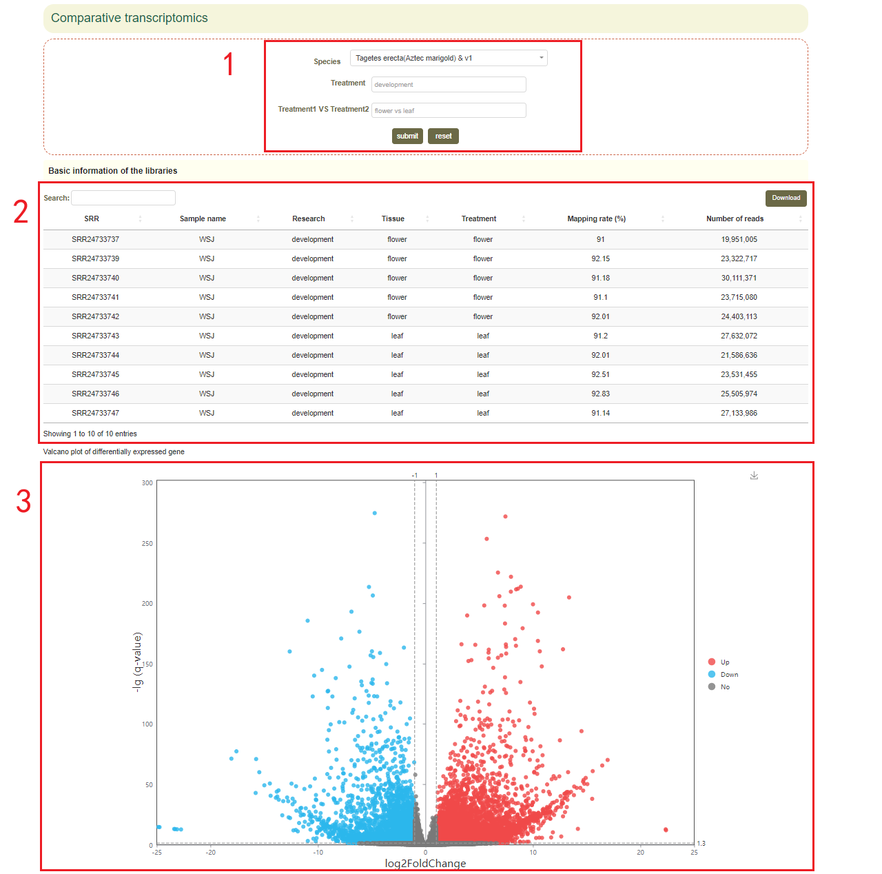
3.4 Differential expression analysis

In this module, comparative transcriptomics analyses related to tissue development, biotic / abiotic treatments, and various stress environments to identify differentially expressed genes under these conditions.

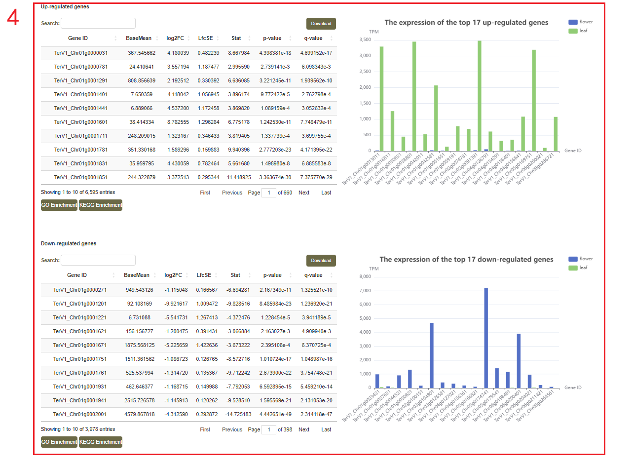
After choosing the "Treatment" and "Treatment group" (box 1), users can first browse the samples applied in this analysis (box 2). Then, the differentially expressed genes can be represented by volcano plot(box 3). The top 20 up/down-regulated genes with the smallest P value are also represented (box 4).

3.5 About

In the “Transcriptomics” module, more than 3,897 RNA-seq libraries corresponding to 131 diverse organs, tissues, and treatments across 44 species have been processed. The portal includes four functional modules, which are single/multiple-species gene expression profile, tissue-specific expressed genes, and comparative transcriptomics. Using this portal, users can analyze and compare 3,897 gene expression profiles, pinpoint genes expressed specifically in certain tissues, and mine differentially expressed genes related to key traits or biological processes.

The quality of the RNA sequencing reads was examined by FastQC (v0.11.9) (https://www.bioinformatics.babraham.ac.uk/projects/fastqc/). Barcode adaptors and low-quality reads (read quality < 70 for paired-end reads) were removed by fastp (v.0.23.0) ^[1]. Then, the filtered reads were aligned to the reference genomes, separately, using Hisat2 (v2.1.0) ^[2] with default parameters. Bam files containing aligned reads were inputted into StringTie (v1.3.3b) ^[3] to measure the expression level of genes. Gene-level raw count data files were generated using featureCounts (v1.6.4) ^[4]. The raw count data were imported into Bioconductor package DESeq2 ^[5] in the R language to identify the differentially expressed genes. Genes had a log2-converted fold change ≥ 1 or ≤ -1 with an FDR (False Discovery Rate) ≤ 0.05 were considered as DEGs.

3.6 References

4. Pathway & Network (Tutorial video)

The following tutorial video will provide a comprehensive overview of this module.

Alternatively, users can explore the tutorial below to learn about the functionality of this module.

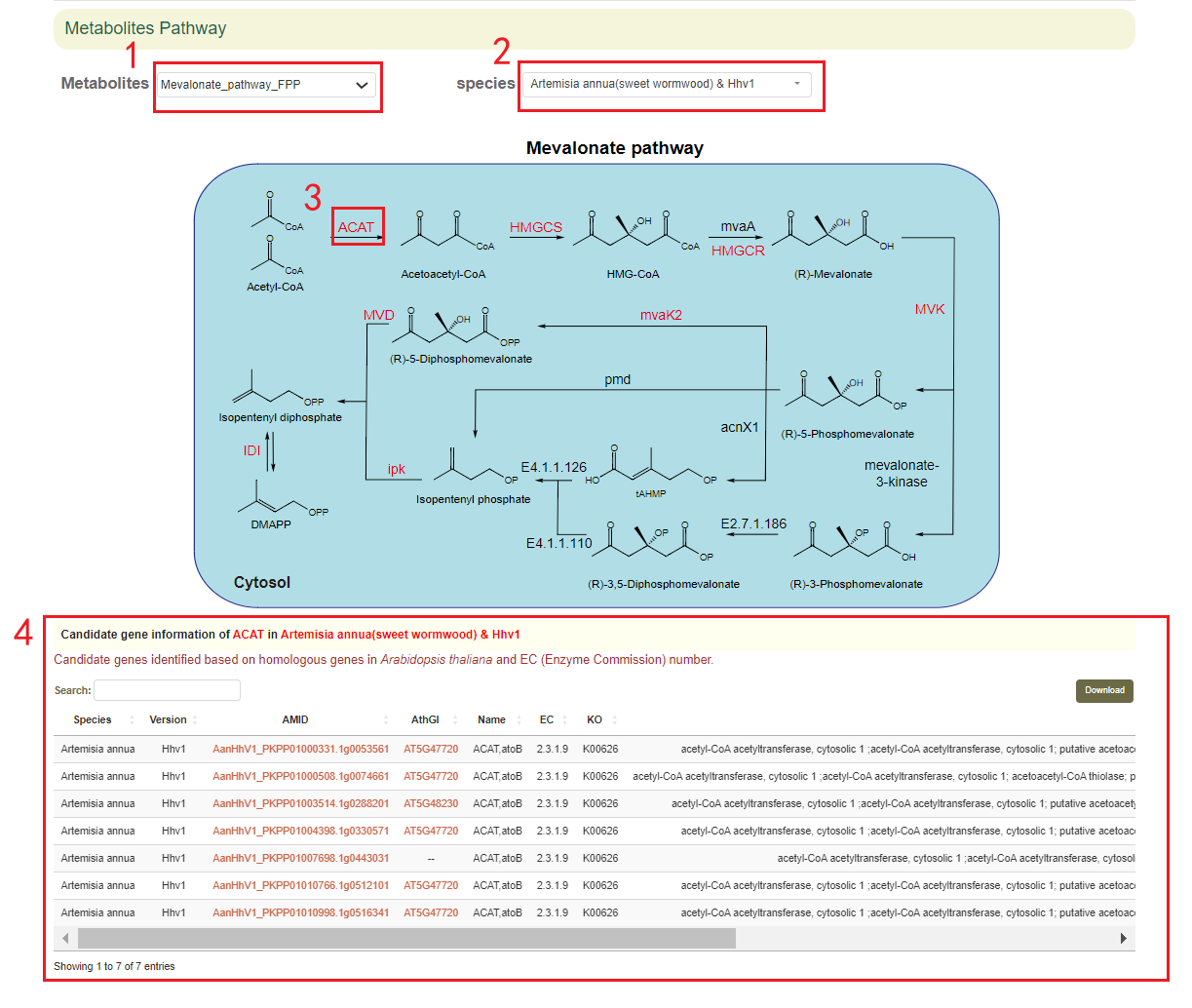
4.1 Secondary Metabolites Pathway

The Secondary Metabolites Pathway module provides eight interactive SVG maps, which were designed for exploring candidate genes involved in the biosynthesis of terpenoid, costunolide, artemisinin, chicoric acids and cyanidin. The user can select the metabolic pathways(box 1) and species(box 2) of interest, and the user obtains the corresponding candidate genes(box 4) in the species by clicking on the key nodes(box 3) of these metabolic pathways.

4.2 KEGG Pathway

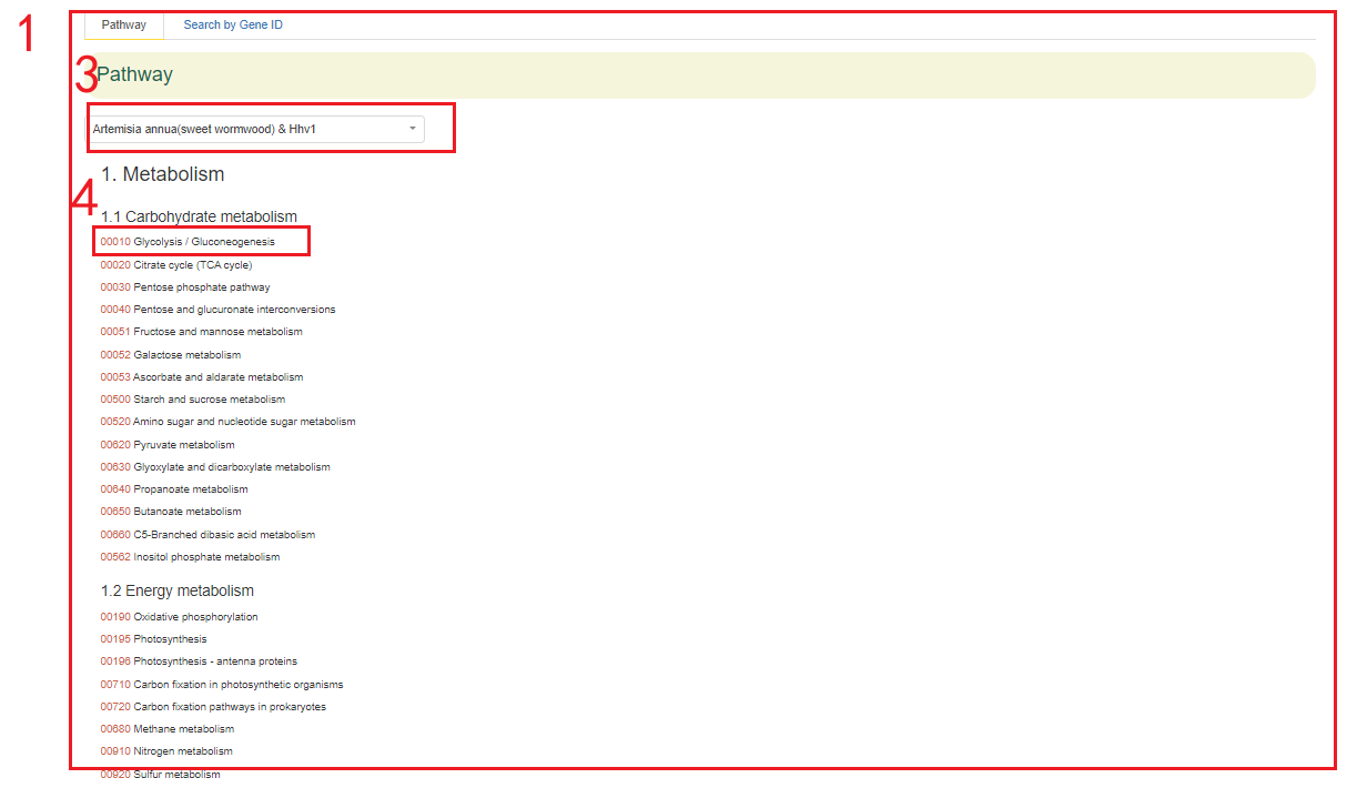
In the KEGG Pathway module, we provide pathway information for the 68 genomes from 54 species within the Asteraceae family. Users can select the pathway of each genome to query the pathway map and the genes related to metabolites.

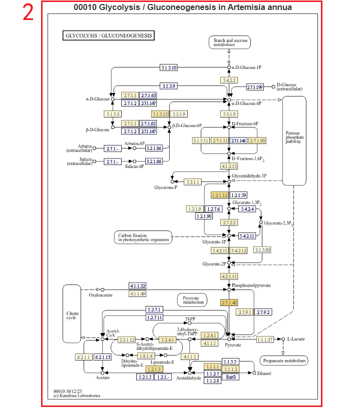
For instance, users can choose the Artemisia annua Hhv1 genome in box 3, and the pathway of the selected genome will be displayed below. By clicking on the pathway number in box 4, the results will appear in box 2. In box 2, different-colored boxes represent the number of genes associated with different metabolites in this genome. Hovering the mouse over a box allows users to view the list of genes related to the corresponding metabolite.

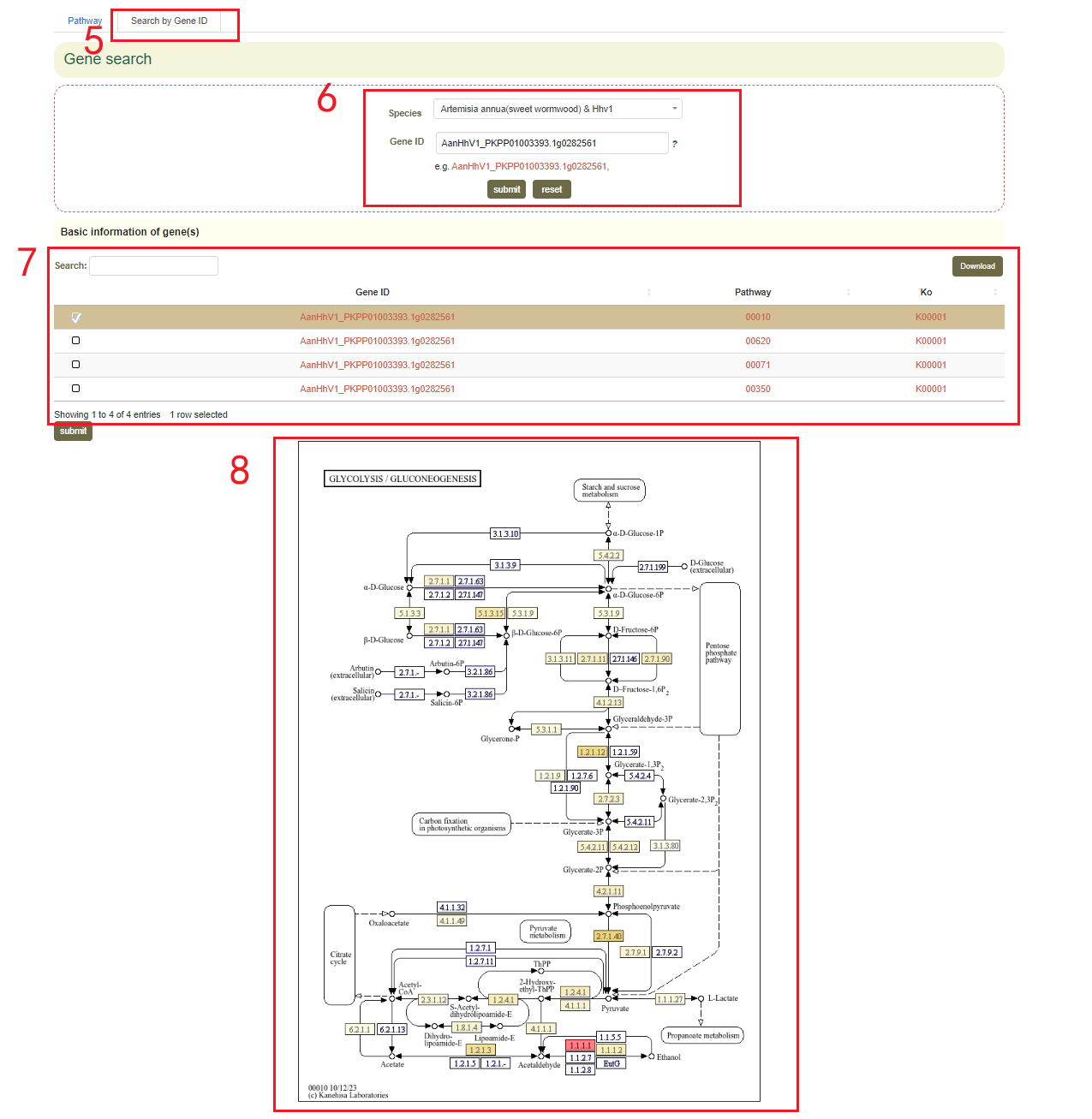
Additionally, users can also enter a gene ID in the "Search by Gene ID" option to check whether the gene is associated with a metabolite, click KO to obtain information on its location in the pathway(boxes 5-8).

4.3 Co-expression

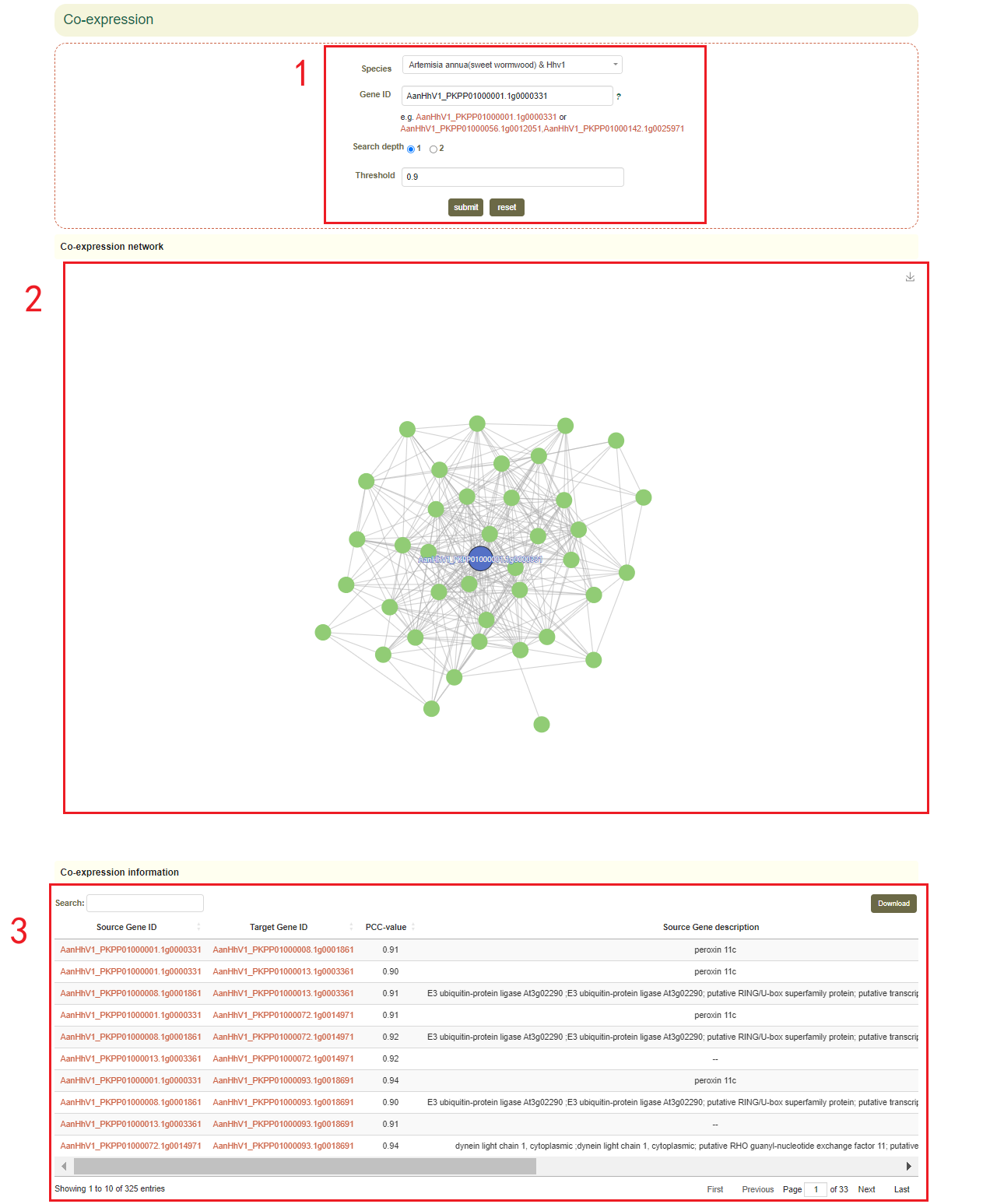
In the Co-expression module, the user first submits one or more gene IDs in the search box, and sets the depth of the network connection (1 or 2) (box1 ), and then clicks “submit” to submit. Next, the user will obtain the co-expression network figure of the gene or genes(box 2) and the pearson correlation coefficients and functional information of the gene or genes(box 3).

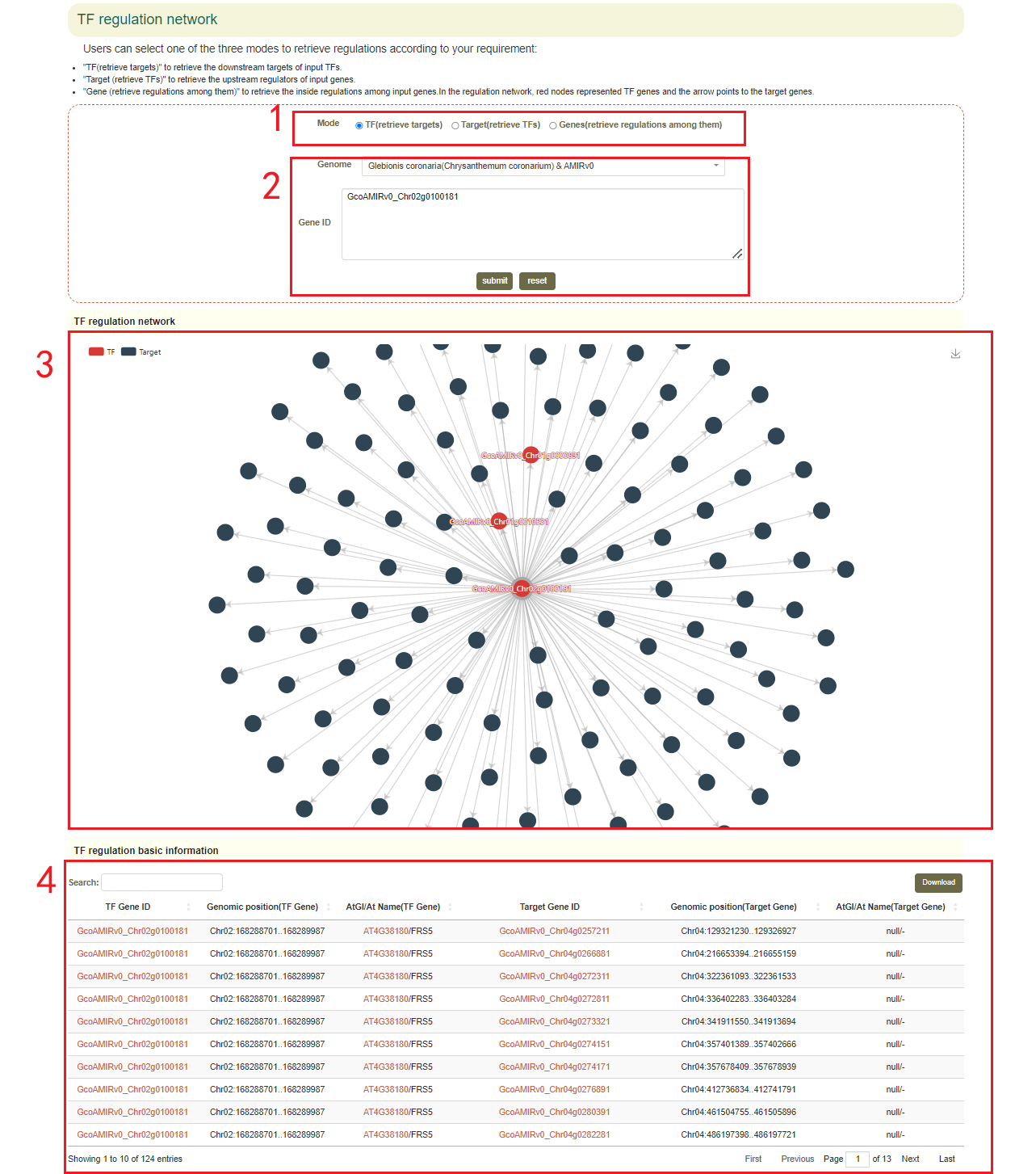
4.4 TF regulation network

In the TF regulation network module, the user first submits one or more gene IDs (box 1) in the search box, and sets the search modes including TF (to retrieve downstream regulated genes), Target (to retrieve the TF genes) or Genes (to retrieve the TF genes and regulated downstream genes)(box 2), and then clicks “submit” to submit. Next, the user will get the network figure of TFs and the target genes(box 3), the pearson correlation coefficients between them and the function information of the genes(box 4).

4.5 About

In the “Pathway” portal, 8 interactive Scalable Vector Graphics (SVG) were designed for exploring candidate genes involved in the biosynthesis of terpenoid, costunolide, artemisinin, chicoric acids and cyanidin. These secondary metabolites are either unique to the Asteraceae or are widely distributed in high concentrations within it. When users hover their mouse over key nodes in different metabolic pathways, the basic information of that gene will be displayed. Clicking on the gene will reveal the corresponding candidate genes in different species. We also added the interactive browsers to explore genes involved in different KEGG pathways (https://www.genome.jp/kegg/).

For the “Network” portal, users can retrieve genes co-expressed with important genes or identify their upstream/downstream regulatory target genes, thereby constructing a gene regulatory network. We have constructed the co-expression module using 74,475,396 co-expression pairs from 31 species. The co-expression network was obtained by calculating the Pearson correlation coefficient (r²) of the gene pairs side by side, and the final gene pairs r² > 0.8 were retained. Finally, we obtained 74,475,396 co-expressed gene pairs.

Furthermore, by using the regulatory prediction function in PlantRegMap ^[1] (https://plantregmap.gao-lab.org/regulation_prediction.php) and based on the regulatory network of Arabidopsis, the transcription factor regulatory networks for 54 species were predicted. The results yielded a total of 1,061,714 TF-gene regulatory pairs.

4.6 References

Tian, F., Yang, D.C., Meng, Y.Q., Jin, J. and Gao, G. (2020) PlantRegMap: charting functional regulatory maps in plants. Nucleic Acids Res, 48, D1104-D1113

5. Tools

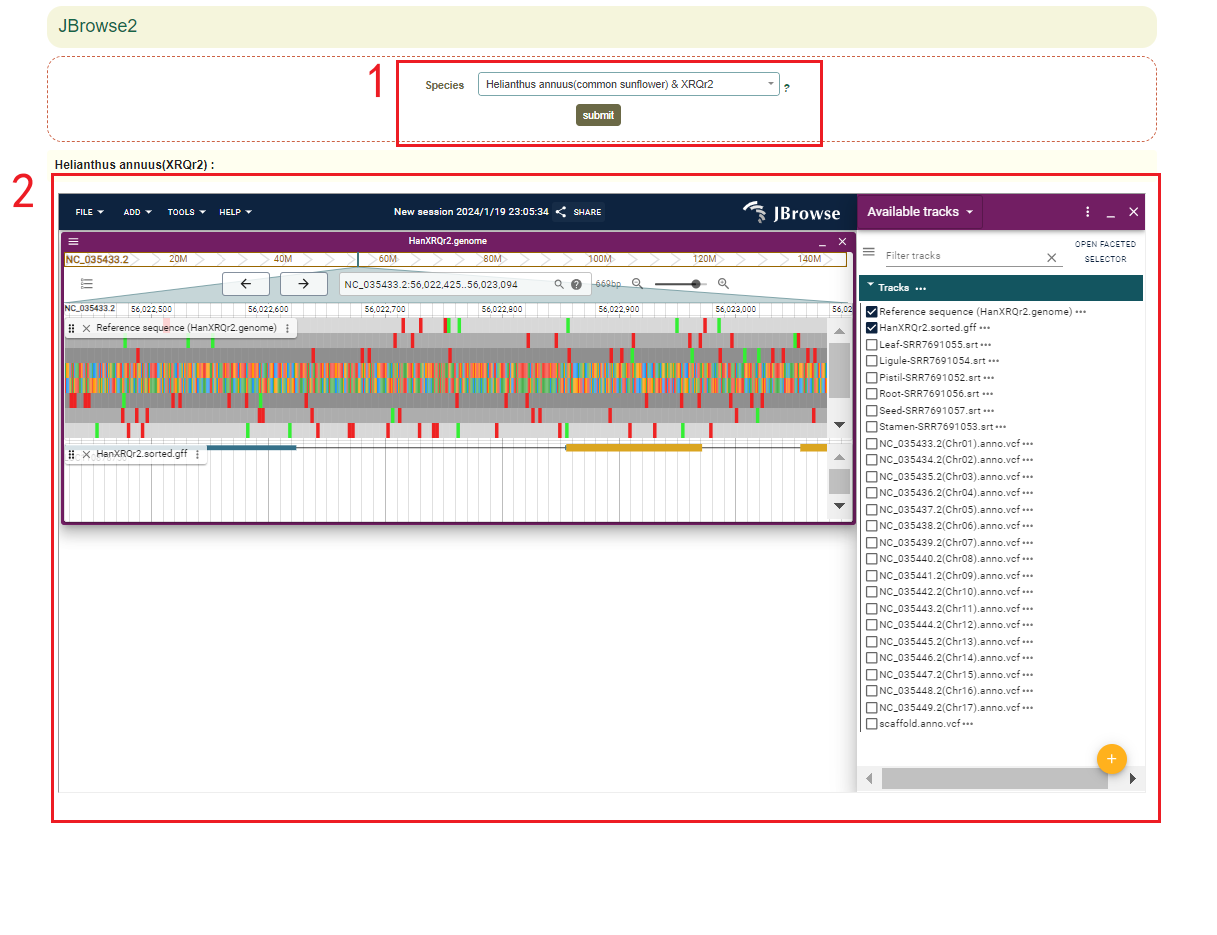
5.1 JBrowser

In JBrowser module, the 68 genome assemblies from 54 species within the Asteraceae family were provided in Jbowser. Fristly,users select the genome assembly(box 1), and then users can visualize the genomic data in the Jbrowse(box 2).

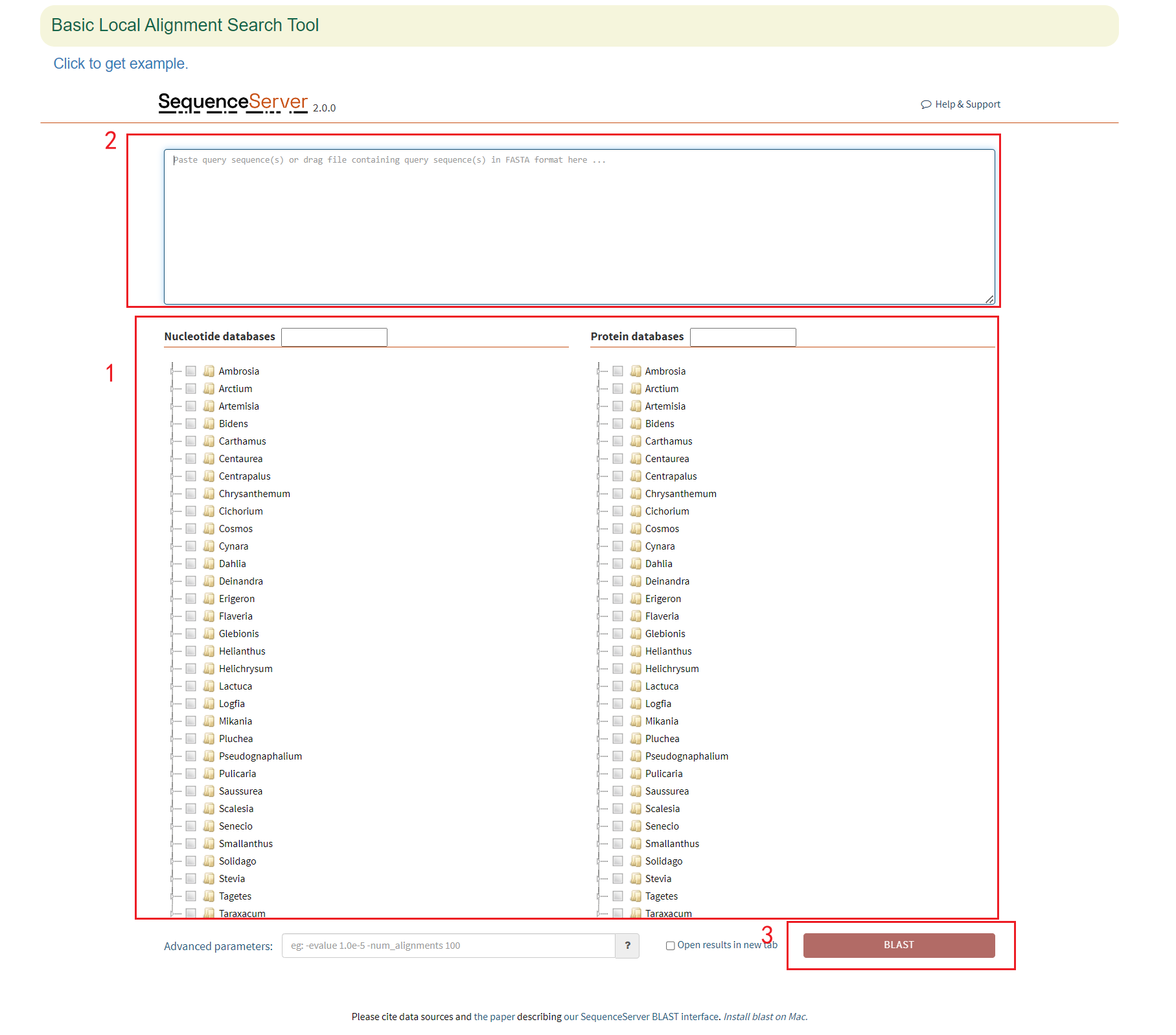
5.2 Blast

In Blast module, the 68 genome assemblies from 54 species within the Asteraceae family were provided. Their genomes, CDS, protein and gene sequences were used to construct the blast library.

The BLAST was based on the SequenceServer application and users can run blast in the following three steps.

Click the circle in front of the genome assembly and sequence to select the genome and sequence type;
Paste the sequence to be queried in the sequence box below;
Select the database type and click 'Submit' to submit.

The first is a graphical representation of the genomic positions to which the sequences are aligned. Then there is a list of all the aligned positions, and the user can click them to query the detailed sequence alignment.

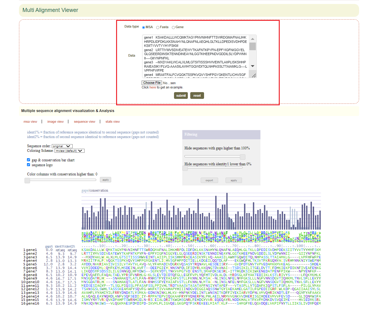
5.3 Multi Alignment Viewer

Enter gene gene list or sequence file, then raw output of result, including visualization of sequences.

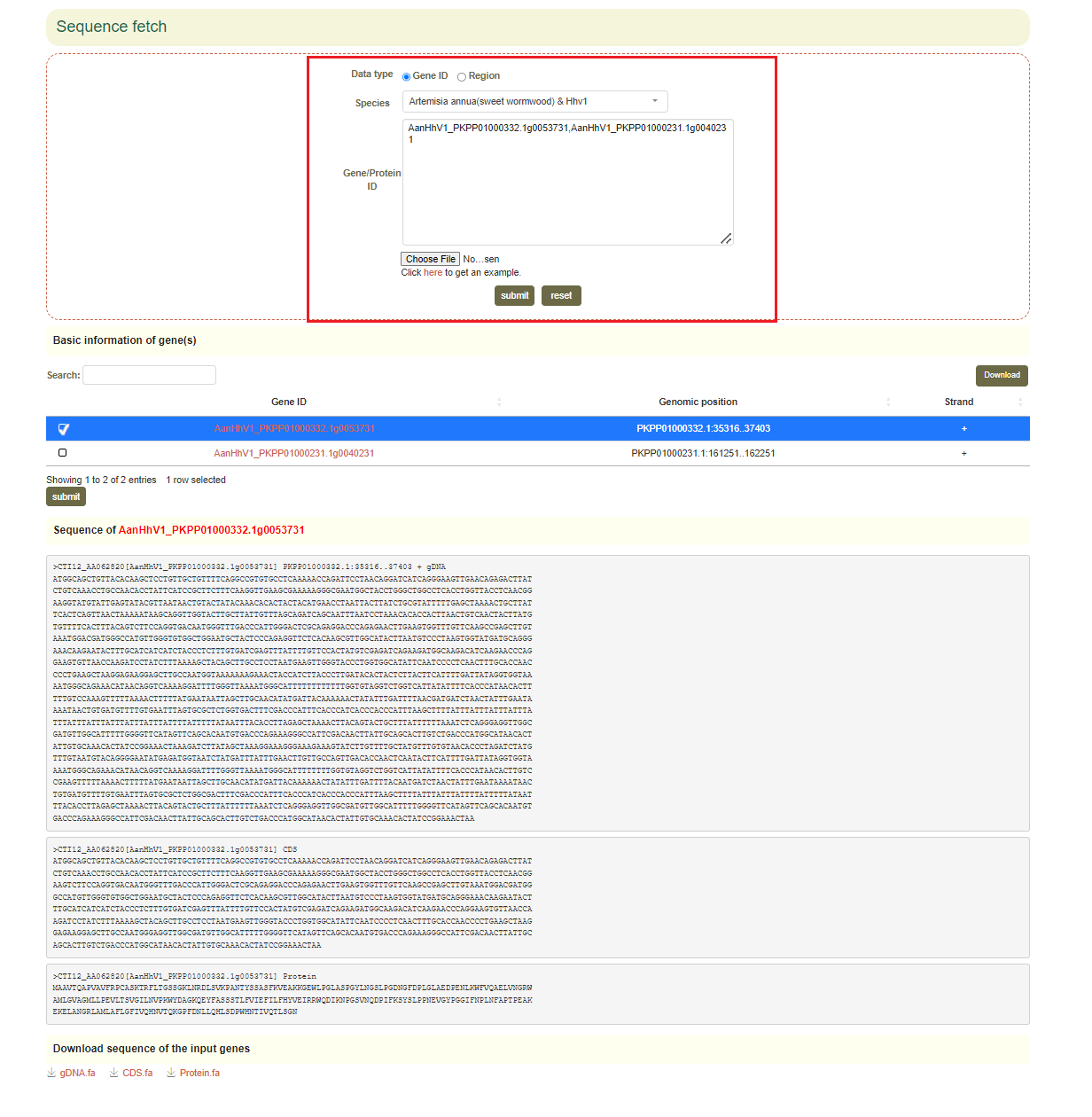
5.4 Sequence fetch

Usage: Paste the gene list to be aligned in the sequence box or upload the gene list file to be extracted and click "Submit" to submit.

Results: You can directly copy the sequences extracted from the dialog box or click on "CDS", "gDNA" and "Protein" in "Download Sequences of all Input Genes" to download these sequences.

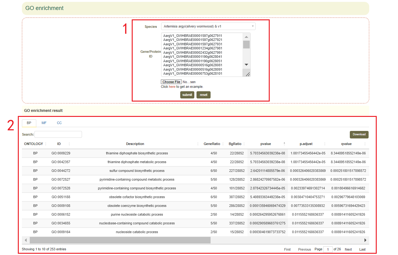
5.5 GO enrichment

Usage:

Paste the gene list in the sequence box or upload the gene list file, and click the "Submit" button.

Results:

1. List of results of GO enrichment analysis. You can switch the category of GO by clicking BP, MF and CC above, and click "Download" in the upper right to download(box 2);

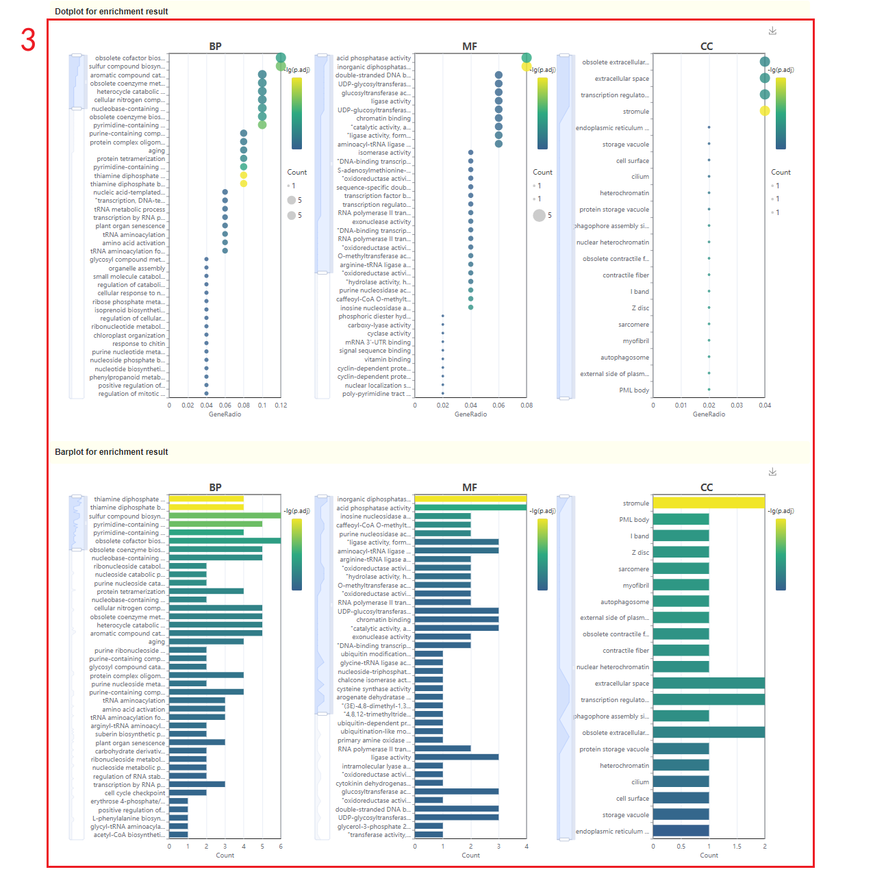
2. The dot plot and bar plot of GO enrichment analysis results. Move the mouse over the figure to query the statistics of the corresponding GO enrichment analysis results. Click the arrow at the top right to download the image(box 2).

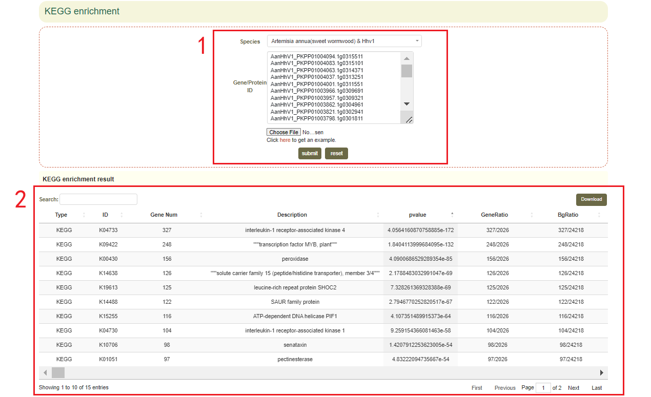
5.6 KEGG enrichment

Usage:

Paste the gene list in the sequence box or upload the gene list file, and click "Submit" to submit.

Results:

1. The result list of KEGG enrichment analysis. Click “Download” in the upper right to download(box 2);

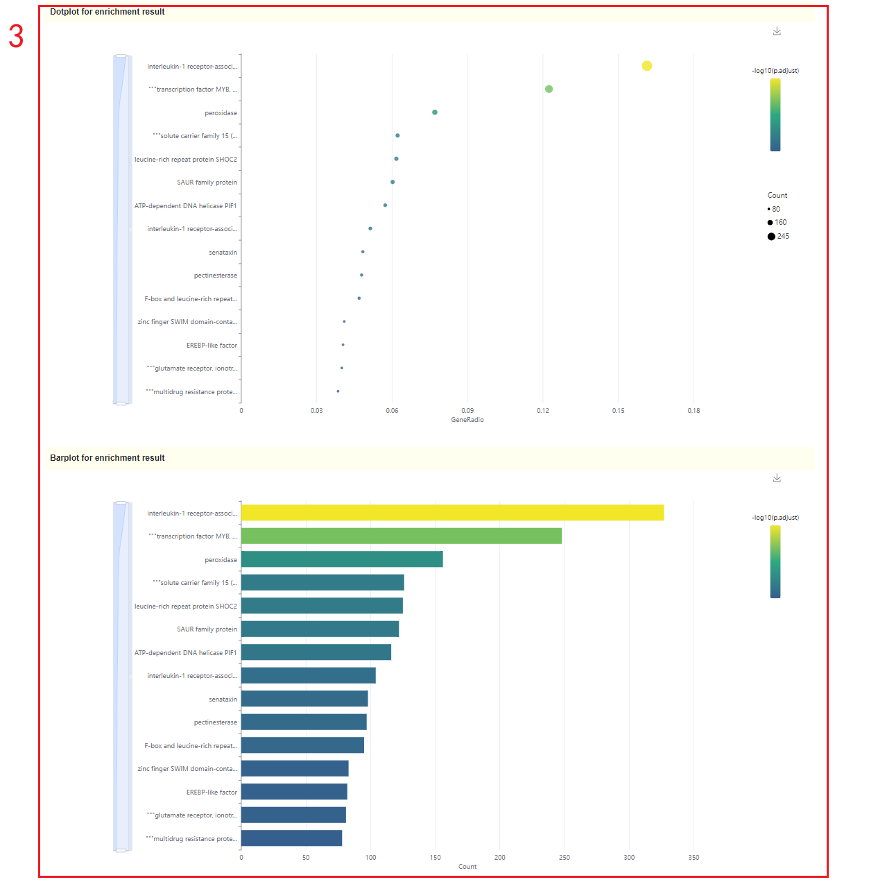
2. Dot plot, bar plot and network plot of KEGG enrichment analysis results. Move the mouse over the figure to query the statistics of the corresponding KEGG enrichment analysis results. Click the arrow at the top right to download the image(box 3).

5.7 Primer3

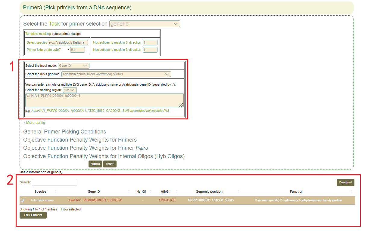
Usage:

1. Select the genome and enter gene ID, genomic region, or upload gene list(box 1);

2.Click "More config" to change the parameters;

3.Click "Submit" to submit;

4.Click "Pick Primers".

Results:

1. 1.Users can obtain the basic information of gene(s)(box 2).

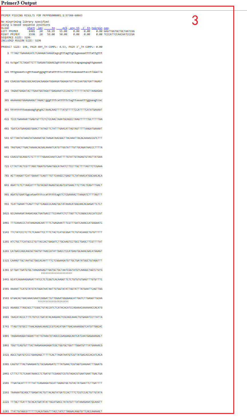
2. After click “Pick Primers”, users can gain the raw output of Primer3, including visualization of primer sequences and their positions on the genome(box3).

5.8 e-PCR

Usage:

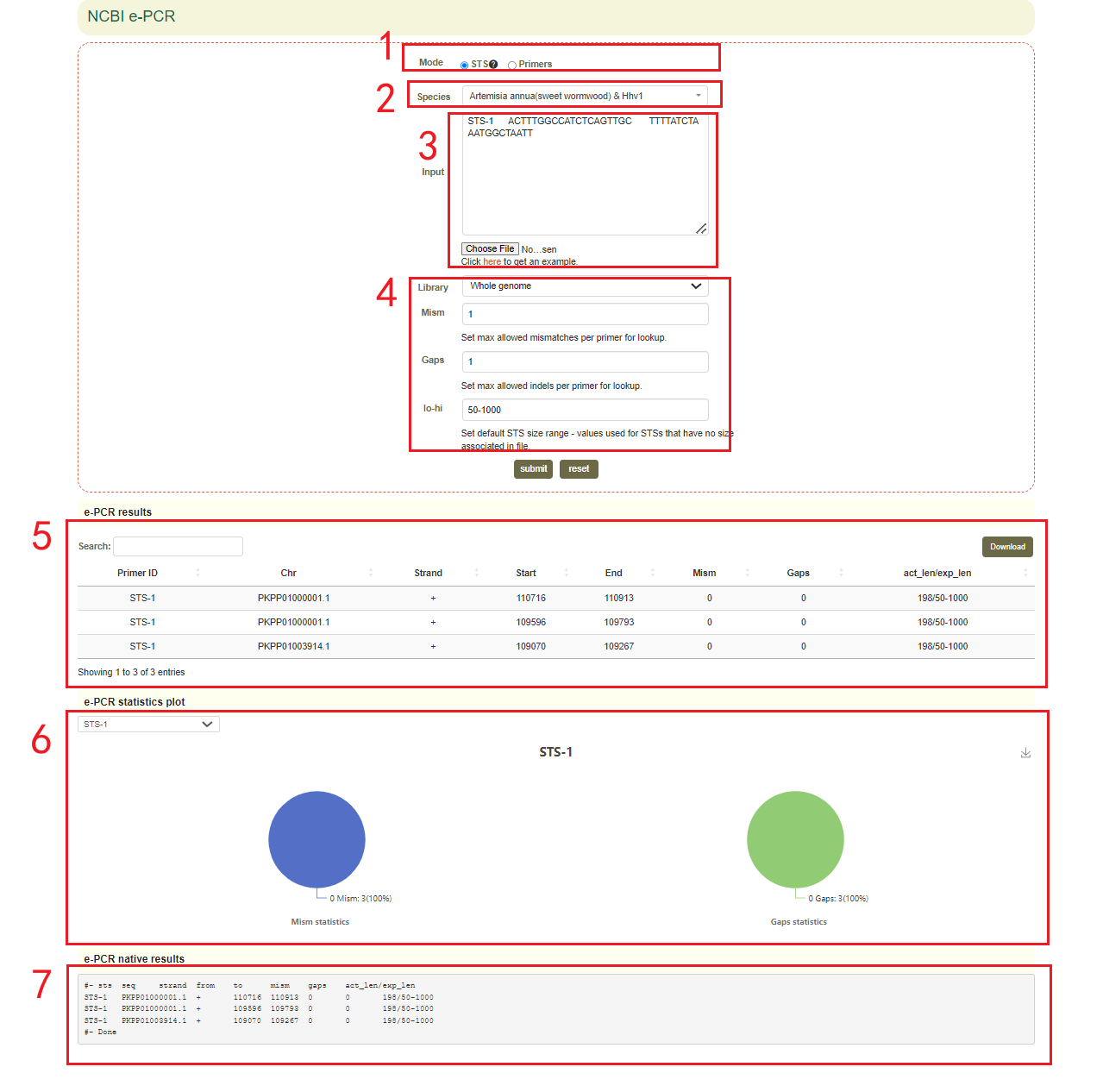
1. Select the file format (STS or Primers) in Mode;

2. Select the genome;

3. Paste the sequence into the dialog or upload the sequence file;

4. Adjust alignment parameters, including mismatch value(mism), gap size(gap) and sequence length range(lo-hi);

Click Submit.

Results:

1. The list of e-PCR results, each row is the position of the sequence amplified by the primers(box 5);

2. Statistical chart of e-PCR comparison results, including the ratio of mismatches and gaps(box 6);

3. The raw output result of e-PCR(box 7).

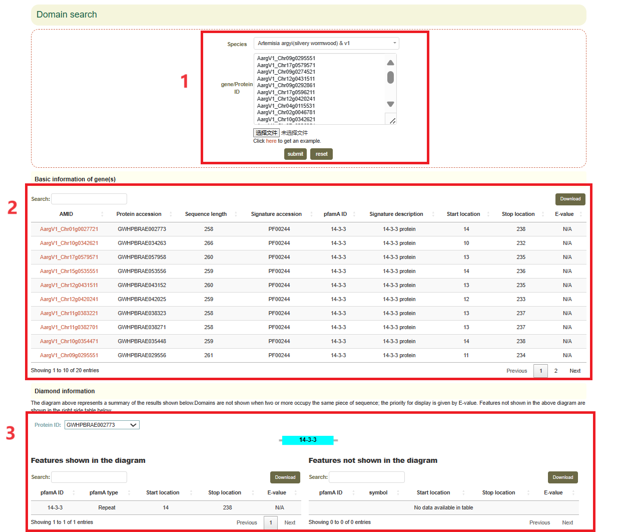
5.9 Domain search

Usage:

1. Select the species and genome in "Species";

2. Paste the gene list in the sequence box or upload the gene list file, and click "Submit" to submit;

Results:

The result list and visualization of Domain. Move the mouse over the figure to see more details.

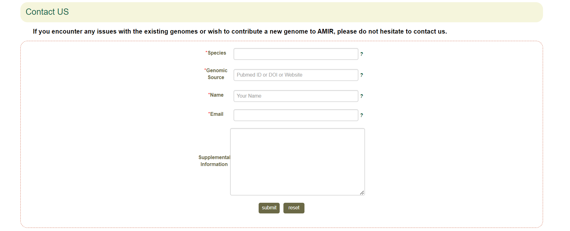
6. Contact Us

6.1 Submit

Furthermore, as a comprehensive platform for Asteraceae Multi-omics Information Resource, we provide a Submit module and plan to continuously update the genome information, maintain and improve the database to better serve the researchers.

7. Database implementation

AMIR was implemented using ThinkPHP framework (v.5.0.24) (https://www.thinkphp.cn/) for its backend. The core JavaScript libraries utilized include Vue.js as the main framework (https://vuejs.org), vis.js for network visualization (https://visjs.org), plotly.js (https://plotly.com), echarts (https://echarts.apache.org), D3.js (https://d3js.org), igv.js (56), and BlasterJS (57) for interactive charts. The system operates on an Apache2 Web server (v.2.4.53) and employs MySQL (v.8.0.29) as its database engine. The database is publicly accessible online without requiring registration and has been optimized for Chrome (recommended), Opera, Firefox, Windows Edge, and macOS Safari. Gene and protein sequence alignment were performed using NCBI BLAST (v.2.13.0+) (58) and MAFFT (v7.490) with parameter “--maxiterate 1000” (59). Genome sequences, gene models, variation and gene expression levels were displayed by JBrowse 2 (60). Web BLAST was driven by Sequencesever (61). Primer design was facilitated using Primer3 (62). Gene set enrichment analysis was conducted using the R package fgsea (63).