1 Comparative genome analysis

Genome sequences were compared between TM-1 reference genome and other 25 genome assemblies using the NUCmer program (v.4.0.0beta2) with parameters "nucmer -- maxmatch -noextend" in MUMmer4. After filtering of the one-to-one alignments with a minimum alignment length of 50 bp using the show-diff program from MUMmer4, the remaining alignment blocks were used for genome browser visualization. For genome browser visualization, dotplot module in JBrowse2 and Genome synteny module in Gbrowser were embedded in CottonMD.

step 1: nucmer --mum --noextend -t $cpu -L 1000 -p $pre $ref $q
step 2: delta-filter -1 -i 95 ${pre}.delta >${pre}.delta
step 3: python $NucDiff/nucdiff.py --proc $cpu --vcf yes --delta_file ${pre}.delta $ref $q $pre $pre

A total of 1,826,981 genes from 25 genome assemblies were used to construct the gene clusters. Firstly, protein sequences of every pair from 25 genome assemblies were aligned using diamond (v.0.9.14.115, http://github.com/bbuchfink/diamond). Then, gene synteny was detected by McScan (python version). The genes with gene synteny were grouped to one cluster. Finally, 1,521,966 genes were grouped to 146,881 gene clusters.

step 1: diamond makedb --in ${i}.pep -d ${i}
step 2: diamond blastp -d ${r} -q ${q}.pep -o ./${q}.${r}.last -f 6 -p 1 -e 1e-5 -k 1 --quiet
step 3: python -m jcvi.compara.catalog ortholog --no_strip_names --cscore=.99 ${q} ${r}
step 4: python -m jcvi.compara.synteny mcscan ${r}.bed ${q}.${r}.lifted.anchors --iter=1 -o ${q}.${r}.i1.blocks

2 SNP and InDel calling

The genome resequencing data of each accession were mapped to the TM-1 reference genome using BWA-MEM with default parameters. Then, the reads with the mapping quality value < 20 were removed by SAMtools (v.1.6). SNPs and small InDels were identified using Sentieon DNAseq pipeline for each accession. SNPs with low mapping quality were filtered out by GATK VariantFiltration with parameters "QUAL < 30.0 || MQ < 50.0 || QD < 2". All SNPs and InDels with minor allele frequencies (MAF) < 0.01 or missing rate > 0.1 were discarded by VCFtools (v.0.1.16). As for the remaining SNPs and InDels, genotype imputation was performed using beagle (v.5.1).

step 1: sentieon bwa mem -R "@RG\tID:${group_prefix}_${i}\tSM:${i}\tPL:$platform" -t $nt -K 10000000 $fasta $fq1 $fq2 | sentieon util sort -r $fasta -o tmp/${i}_q0.bam -t $nt --sam2bam -i -
step 2: samtools flagstat tmp/${i}_q0.bam > 02.FinalBam/${i}.flagstat
        samtools stats -@ $nt tmp/${i}_q0.bam > 02.FinalBam/${i}.stats
        samtools view -h -q 20 tmp/${i}_q0.bam | sentieon util sort -r $fasta -o tmp/${i}_sorted.bam -t $nt --sam2bam -i -
        sentieon driver -r $fasta -t $nt -i tmp/${i}_sorted.bam --algo MeanQualityByCycle tmp/${i}_mq_metrics.txt --algo QualDistribution tmp/${i}_qd_metrics.txt --algo GCBias --summary tmp/${i}_gc_summary.txt tmp/${i}_gc_metrics.txt --algo AlignmentStat --adapter_seq '' tmp/${i}_aln_metrics.txt --algo InsertSizeMetricAlgo tmp/${i}_is_metrics.txt
        sentieon plot metrics -o tmp/${i}_metrics-report.pdf gc=tmp/${i}_gc_metrics.txt qd=tmp/${i}_qd_metrics.txt mq=tmp/${i}_mq_metrics.txt isize=tmp/${i}_is_metrics.txt
        sentieon driver -t $nt -i tmp/${i}_sorted.bam --algo LocusCollector --fun score_info tmp/${i}_score.txt
        sentieon driver -t $nt -i tmp/${i}_sorted.bam --algo Dedup --rmdup --score_info tmp/${i}_score.txt --metrics tmp/${i}_dedup_metrics.txt tmp/${i}.deduped.bam
        sentieon driver -r $fasta -t $nt -i tmp/${i}.deduped.bam --algo Realigner 02.FinalBam/${i}.bam
        samtools idxstats 02.FinalBam/${i}.bam >02.FinalBam/${i}.idxstats
step 3: sentieon driver -r $fasta -t $nt -i 02.FinalBam/${i}.bam --algo QualCal tmp/${i}_recal_data.table
        sentieon driver -r $fasta -t $nt -i 02.FinalBam/${i}.bam -q tmp/${i}_recal_data.table --algo QualCal tmp/${i}_recal_data.table.post
        sentieon driver -t $nt --algo QualCal --plot --before tmp/${i}_recal_data.table --after tmp/${i}_recal_data.table.post tmp/${i}_recal.csv
        sentieon plot bqsr -o tmp/${i}_recal_plots.pdf tmp/${i}_recal.csv
        sentieon driver -r $fasta -t $nt -i 02.FinalBam/${i}.bam -q tmp/${i}_recal_data.table --algo Haplotyper --emit_mode gvcf 03.OriGVCF/${i}_gvcf.gz
        #After all accession have done the above steps
        sentieon driver -r $ref -t $nt --algo GVCFtyper 04.Vcf/${out}.raw.vcf.gz 03.OriGVCF/*_gvcf.gz
step 4: java -Xmx30g -jar ${gatk_path} -T SelectVariants -R ${ref} -V ${vcf} -o ${out}.snp.vcf.gz -selectType SNP -nt ${nt} 
        java -Xmx30g -jar ${gatk_path} -T SelectVariants -R ${ref} -V ${vcf} -o ${out}.indel.vcf.gz -selectType INDEL -nt ${nt}
        java -Xmx30g -jar ${gatk_path} -T VariantFiltration -R ${ref} -V ${vcf}.snp.vcf.gz -o ${vcf}.snp.flt.vcf.gz --filterExpression "QUAL < 30.0 || MQ < 50.0 || QD < 2\" --clusterSize 3 --clusterWindowSize 10 --filterName \"myfilter\“
        java -Xmx30g -jar ${gatk_path} -T VariantFiltration -R ${ref} -V ${vcf}.indel.vcf.gz -o ${vcf}.indel.flt.vcf.gz --filterExpression \"QUAL < 30.0 || MQ < 50.0 || QD < 2\" --clusterSize 3 --clusterWindowSize 10 --filterName \"myfilter\"
step 5: vcftools --vcf ${vcf} --maf 0.05 --max-missing 0.9 --min-alleles 2 --max-alleles 2 --recode --recode-INFO-all --out ${out}
step 6: java -jar beagle.18May20.d20.jar nthreads=20 window=10000 overlap=600 gt=${vcf} out=${out}

3 Transcriptome analysis

After clipping the adaptor sequences and removing the low-quality reads by Trimmomatic software (v.0.36), the RNA-seq clean data from accessions were mapped to the TM-1 reference genome using Hisat2 (v.2.1.2) with default parameters. Gene expression level was normalized using the number of transcripts per kilobase million reads (TPM) by StringTie software (v.1.3.5) with default settings. The co-expression network was obtained by calculating the Pearson correlation coefficient of pairwise gene expression levels, and the gene modules including the gene pairs with a Pearson correlation coefficient of larger than 0.8 were retained as a co-expression network.

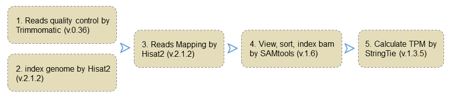
step 1: java -jar trimmomatic-0.36.jar PE -threads $nt $raw_fq1 $raw_fq2 $fq1 $fq1_unpaired $fq2 $fq2_unpaired ILLUMINACLIP:./TruSeq3-PE.fa:2:30:10 LEADING:3 TRAILING:3 SLIDINGWINDOW:4:15 MINLEN:36
step 2: hisat2-build -p $nt ${ref}.fa ${ref}
step 3: hisat2 -p $nt --summary-file 01.bams/${s}_summary.txt --dta -x $ref -1 $fq1 -2 $fq2 | samtools view -Sbho 01.bams/${s}.bam - 1>01.bams/${s}.log 2>01.bams/${s}.err
step 4: samtools sort -@ $nt -o 01.bams/${s}.srt.bam  01.bams/${s}.bam
        samtools index 01.bams/${s}.srt.bam && rm 01.bams/${s}.bam
step 5: stringtie 01.bams/${s}.srt.bam -p $nt -G $gtf -e -B -o 02.stringtie/${s}/${s}.gtf -A 02.stringtie/${s}/${s}.tab -l ${s}

4 Epigenome analysis

The adaptor sequences were removed and the low-quality reads were filtered out using Trimmomatic (v.0.36). As for ChIP-seq and ATAC-seq, the clean data from accessions were mapped to the TM-1 reference genome using bowtie2 (v.2.3.2) with default parameters. PCR duplicated reads were removed using Picard tools (v.2.19). Peaks were called using the callpeak module of MACS2 software (v.2.1.2) with the parameters " --broad -f BAM -g 2290000000 -B -p 0.00001 --nomodel --extsize 147 ".

step 1: java -jar trimmomatic-0.36.jar PE -threads $cpu ./${i}_R1.fastq.gz ./${i}_R2.fastq.gz ./${i}_1.fq.gz ./${i}_unpaired_1.fq.gz ./${i}_2.fq.gz ./${i}_unpaired_2.fq.gz ILLUMINACLIP:./TruSeq3-PE.fa:2:30:10 LEADING:3 TRAILING:3 SLIDINGWINDOW:4:15 MINLEN:36
step 2: bowtie2 -x $ref -p $cpu -U 01.trim/${i}.fq.gz |samtools view -bS -o 02.bam/${i}.raw.bam
step 3: samtools flagstat 02.bam/${i}.raw.bam > 02.bam/${i}.bowtie2.log
step 4: samtools view -bh -o 02.bam/${i}.bam -q 10 02.bam/${i}.raw.bam
step 5: samtools sort -@ $cpu -o 02.bam/${i}.sort.bam 02.bam/${i}.bam
step 6: samtools index 02.bam/${i}.sort.bam && rm 02.bam/${i}.raw.bam 02.bam/${i}.bam
step 7: macs2 callpeak -t ${treat}.sort.bam -c ${control}.sort.bam  --broad -f BAM -g 2290000000 -n $4 -B -p 0.00001 --nomodel --extsize 147 --outdir 03.macs/
step 8: macs2 bdgcmp -t 03.macs/${n}_treat_pileup.bdg -c 03.macs/${n}_control_lambda.bdg --outdir 03.macs/ -o ${n}_PE.bdg  -m FE
step 9: bedGraphToBigWig 03.macs/${n}_PE.bdg ref/TM-1.genome.fa.fai 03.macs/${n}_PE.bw

As for Hi-C, the clean reads of each accession were mapped to the TM-1 reference genome using BWA-MEM with default parameters. Then, the Hi-C interaction matrix was created using Juicer pipeline. KR normalized matrix was extracted from Hi-C format files at the resolutions of 10 kb, 50 kb and 100 kb using Juicer_tools (v.1.7.6) for JBrowser.

step 1: ~/juicer/CPU/juicer.sh -g $r -s DpnII -p ${r}.chrom.sizes -y ${r}_DpnII.txt -z ${r}.fa -D ${HOME}/juicer/CPU -t 40
step 2: java -jar ~/bin/juicer_tools.jar dump observed NONE ${i}.hic $chri $chrj BP $reso ${chri}_${chrj}.txt

As for BS-seq data, clean data of each accession were mapped to the TM-1 reference genome using Bismark (v.0.13.0) with parameter settings "-N 1, -L 30". Bigwig files of all epigenome data analysis can be visited by JBrowser in the Tools portal.

step 1: bismark --genome $ref_dic --path_to_bowtie2 /home/share/bin -1 ./02.Cleandata/${i}_1.fastq.clean.gz -2 ./02.Cleandata/${i}_2.fastq.clean.gz -p $nt -N 1 -L 30 -o ./03.Bam 2>log/${i}_bowtie2.map.log;
step 2: deduplicate_bismark  --outfile $i --output_dir ./03.Bam --paired ./03.Bam/${i}_1.fastq.clean.gz_bismark_bt2_pe.bam 2>log/${i}_deduplicate.log
step 3: bismark_methylation_extractor --no_overlap -o ./04.Extractor --parallel $nt --gzip --bedGraph --buffer_size 10G --CX --cytosine_report --genome_folder $ref_dic 03.Bam/${i}.deduplicated.bam 2>log/${i}_extracor.log

5 Population genetic analysis

SNPs and InDels were filtered based on linkage disequilibrium (LD) using PLINK (v.1.90b4.4) with the parameters "--indep-pairwise 100 50 0.8". Variations passing filtering were used for the downstream analysis. Phylogenetic tree of 4,180 cotton accessions was constructed using FastTreeMP (v.2.1) with the default parameters. Population structure of all accessions was analyzed using fastStructure with K from 2 to 10. Principal component analysis (PCA) was performed using GCTA (v.1.92.4 beta2).

step 1: plink --bfile ${i} --indep-pairwise 100 50 0.8 --out ${i} --autosome-num 26
step 2: plink --bfile $pre --extract ${i}.prune.in --recode --out LD_chrs/${i}.pruned --allow-extra-chr
        python ~/code/ped2fa.py ${out}.pruned.ped ${out}.pruned.fa
        #Phylogenetic tree
step 3: FastTreeMP -nt -gtr ${out}.pruned.fa > ${out}.pruned.fastreee.tree
        #Population structure
step 4: i=cotton4180.pruned
        out=Q/cotton4180.pruned
        python ~/fastStructure/structure.py -K 2 --input=$i --output=$out &
        python ~/fastStructure/structure.py -K 3 --input=$i --output=$out &
        python ~/fastStructure/structure.py -K 4 --input=$i --output=$out &
        python ~/fastStructure/structure.py -K 5 --input=$i --output=$out &
        python ~/fastStructure/structure.py -K 6 --input=$i --output=$out &
        python ~/fastStructure/structure.py -K 7 --input=$i --output=$out &
        python ~/fastStructure/structure.py -K 8 --input=$i --output=$out &
        python ~/fastStructure/structure.py -K 9 --input=$i --output=$out &
        python ~/fastStructure/structure.py -K 10 --input=$i --output=$out &
        #PCA
step 5: gcta64 --bfile cotton4180.pruned --autosome --make-grm --out cotton4180.pruned
step 6: gcta64 --grm cotton4180.pruned --pca 10 --out 

6 Genome-wide association study (GWAS)

The SNPs and InDels with a minor allele frequency (MAF) of lower than 5% were filtered for genome-wide association study (GWAS). GWAS was performed for six traits using the GEMMA (v.0.98.1). The population structure was controlled by including the first two principal components as covariates, as well as an IBS kinship matrix derived from all variants (SNPs and InDels) calculated by GEMMA. The cutoff for determining significant associations was set as -log10(1/n), where n represents the total number of variations.

step 1: vcftools --gzvcf $vcf --maf 0.05 --min-alleles 2 --max-alleles 2 --recode --recode-INFO-all --out ${out}_maf0.05
step 2: plink --vcf ${out}_maf0.05.recode.vcf --make-bed --out ${out}
step 3: gemma -bfile $f -k $kin -lmm 1 -c $q -o ${out}_${p} -p ${p}.txt

7 Expression quantitative trait loci (eQTL) mapping

The gene expression values were taken as the values of the phenotype for eQTL mapping. Only those genes expressed in more than 95% of the accessions were defined as expressed genes for eQTL mapping. Variations with MAF > 5% were used to perform GWAS for each gene by using GEMMA to detect the associations for variations and genes. The cutoff for determining significant associations was set as -log10(1/n), where n represents the total number of variations. Then, eQTL mapping was performed as previously described. Based on the distance between eQTL and targeted-genes, we subdivided all eQTL into cis-eQTL if the variation was found within 1 Mb of the transcription start site or transcription end site of the target gene, otherwise as trans-eQTL. In CottonMD, the regulatory relationship of trans-eQTL was visualized using BioCircos.js.

step 1: vcftools --gzvcf $vcf --maf 0.05 --min-alleles 2 --max-alleles 2 --recode --recode-INFO-all --out ${out}_maf0.05
step 2: plink --vcf ${out}_maf0.05.recode.vcf --make-bed --out ${out}
step 3: gemma -bfile $f -k $kin -lmm 1 -c $q -o ${out}_${p} -p ${gi}.txt

8 Transcriptome-wide association studies (TWAS)

TWAS was used to integrate GWAS and gene expression datasets to identify gene-trait associations. TWAS was conducted by the EMMAX module using the gene expression data of fiber at 20 DAP with the data of six phenotypes from cis-eQTL in the region of 1 Mb upstream to 1 Mb downstream of target genes to compute the gene expression weights. Models were considered as 'transcriptome-wide significant' if they passed the Bonferroni correction for all genes.

9 Colocalization analysis

Colocalization of GWAS and eQTL results was performed to generate posterior causal probabilities for each of the variants in the GWAS and eQTL analyses. All variations within 1 Mb flanking region around the gene were tested for colocalization using the "COLOC" R package with default parameters. The variants in cis-eQTLs of genes and QTLs of phenotypes were defined as colocalized when the posterior probability of a colocalized signal (PPH4) value was larger than 0.5 and there is at least one shared significant variation.

10 SMR analysis

SMR analysis integrated the summary-level data from GWAS with eQTL data to identify genes associated with a complex trait because of pleiotropy. The cis-eQTL signals of expressed genes and GWAS signals of the phenotype were used to perform SMR analysis and HEIDI test by SMR software(v.1.03). Then, the gene was defined to be a candidate gene of the phenotype when -log10(P-value) of SMR was less than 3.77 (1/n, n is the number of all expressed protein-coding genes) and P-value of HEIDI test was larger than 0.01.

smr_Linux --bfile $fi --gwas-summary GWAS_summary/${i}.ma --beqtl-summary $eqtl --out ${i} --thread-num 10 --disable-freq-ck