Genomics
Gene search
The Gene search page provides gene structure and function information of ZS11 and Darmor genomes. In this module, the user can enter the gene ID of ZS11 or Darmor to query the related information of the interest gene. If users entered the gene ID or gene name of Arabidopsis thaliana, the structure and function information of all homologous genes and their phylogenetic relationship can be obtained.
For example, if users entered 'AT1G65480'(box 1), users can obtain the physical location and functional description information of all homologous genes corresponding to this gene (box 2 and box 3), the phylogenetic relationship of homologous genes (box 4).

Gene cluster
Gene cluster provides a query of gene cluster results for 11 rapeseed genomes. The user can query the copy number of the genes by entering the Arabidopsis Gene ID or Gene name.
For example, if users entered 'AT1G65480' at box 1, results in boxes 2-5 will be obtained. The gene IDs of different genome assemblies corresponding to the gene cluster where the gene is located can be obtained in box 2; the copy number difference of the gene cluster in all genomes is listed in box 3; the functional description of the genes in this gene cluster is given in box 4; the physical location information of the genes in this gene cluster will be obtained in box 5.
Gene family
Gene family integrates information from 181 gene families. In this module, the user can select a gene family to query for ZS11 genes information, ZS11 genes copy number transformation, and ZS11 genes copy number distribution for that gene family. box 1 lists each gene family is listed. If users select and submit '14-3-3 proteins' at box 1, the gene list of the corresponding gene family and the statistics of the copy number of B. napus genome corresponding to the Arabidopsis genes in this family will be obtained (box 2).
Gene index
Gene index constructed a total of 88,423 gene indexes by integrating the gene collinearity of 11 B. napus genomes. By entering the Arabidopsis gene ID, gene name or the gene ID of the B. napus genome (box 1), users can view the gene index of related genes (box 2).
Genome synteny
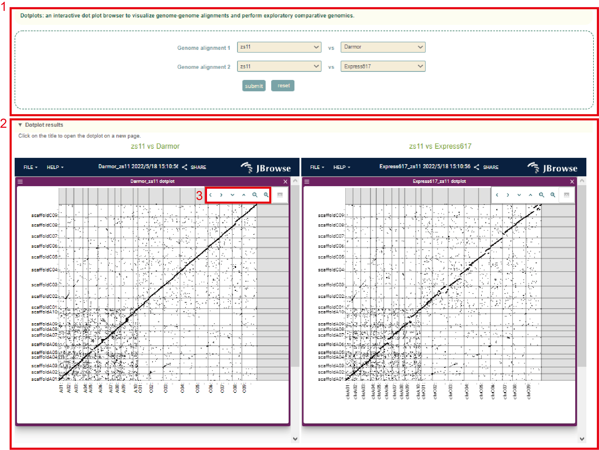
We collected 14 genome assemblies including the diploids Brassica rapa accessions Chinese cabbage Chiifu-401-41, sarson Z1, Brassica oleracea accessions HDEM, To1000, and 11 Brassica napus accessions. By genome alignment, genomic synteny was constructed. We integrated Gbrowser_syn and Dotplot browsers to browse the genome alignments. The Dotplots browser can help users browse the global and local genome collinearity between genome assemblies. In Dotplots, users are allowed to browse the collinearity between two genome alignments simultaneously. The user selects the object of the gene alignment to be viewed in box 1, and then gets the genome collinearity result in box 2, and can browse by switching the position and resolution of the genome in box 3 .
Users can browse the alignment results of all regions between genomes using Gbrowser_syn. In Gbrowser, the user selects the object of the gene alignment to view(box 1), and then gets the result(box 2). The genomic collinearity (box 6) is finally obtained by selecting the reference genome (box 3), the genomic region to be viewed(box 4), and the resolution(box 5).

Pan-browser
Pan-browser is a Jbrowser of Brassica napus pangenome. The operation guide of Jbrowser can be found here.
Pathway
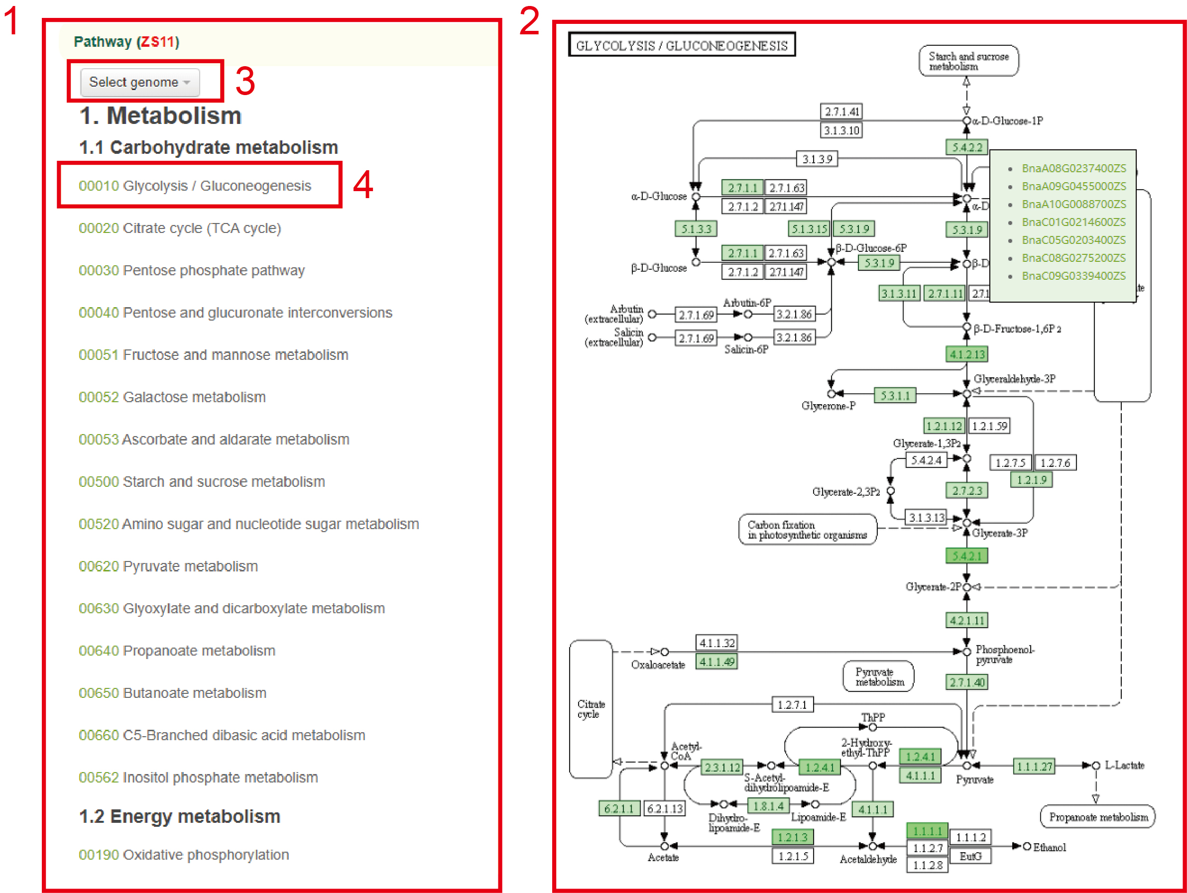
In the Pathway module, we provide the pathway information of seven B. napus genomes. In this module, users can select the pathway of each genome to query the map of the pathway and the genes related to metabolites.
For example, users can select the ZS11 genome in box 3, and the pathway of the selected genome will be displayed below. After clicking the pathway number in box 4, the results will be displayed in the box 2. In box 2, The boxes with different colors indicate the number of genes corresponding to different metabolites in this genome. By hovering the mouse over the box, you can view the list of genes related to the metabolite.
Transcription factor(TF)
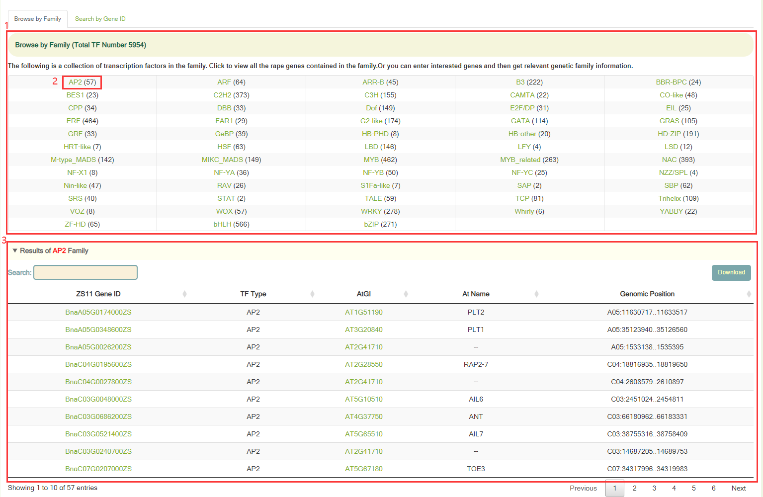
In Transcription factor module, we annotated a total of 5,954 genes encoding transcription factors in 58 families based on the TF information in the Arabidopsis genome and the homologous gene relationship between ZS11 and Arabidopsis genomes.
Users can browse the number of genes in all gene families using "Browse by Family" (box 1), and view the number of genes in that family by clicking on the gene family name. For example, when you click on AP2 (box 2), you will get a list of genes belonging to this family (box 3). In addition, users can also enter the gene ID in "Search by Gene ID" to check whether the gene is a transcriptome factor and its gene family information.
Population
Population information
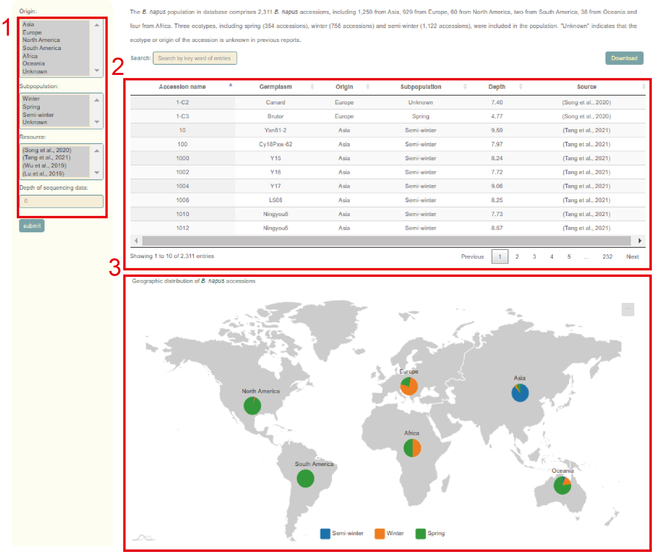
In the Population information module, users can query the related information of the collected 2311 Brassica napus accessions. Users can filter accessions according to their Origin, Subpopulation, Resource, and sequencing depth (box 1). Then, the user will get information such as germplasm name, geographic origin, subgroup, sequencing depth, and data source of these accessions (box 2), as well as the proportion of accessions from different subpopulations on each continent (box 3).
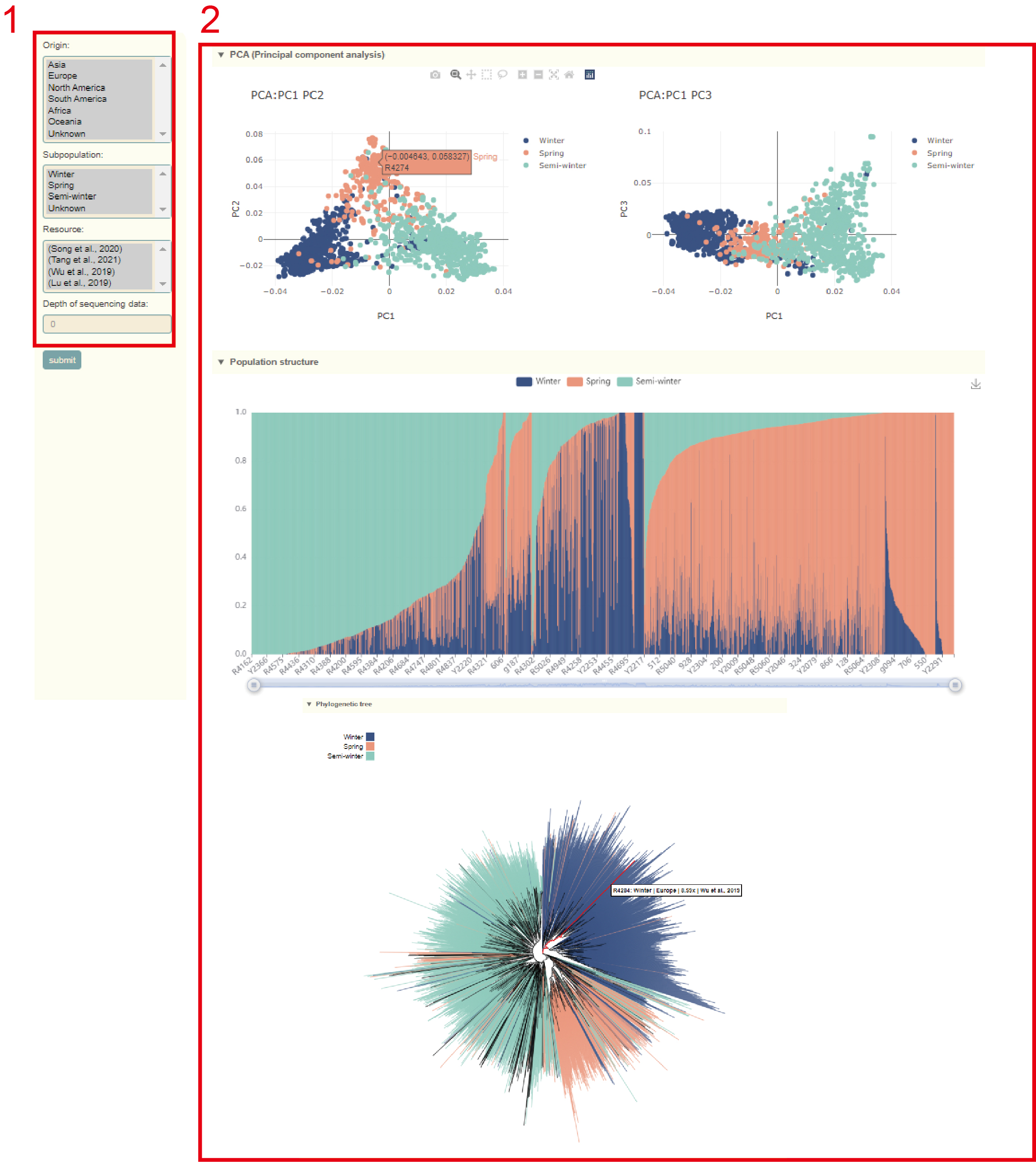
Population structure
In the Population information module, users can query the population structure information of the 2311 Brassica napus accessions. Users can filter accessions according to their Origin, Subpopulation, Resource, and sequencing depth (box 1). Then, users can obtain the results of PCA, population structure analysis, and phylogenetic analysis of these accessions (box 2). The user can move the mouse over these points or columns to query the population structure information of this accession.
Selective signals
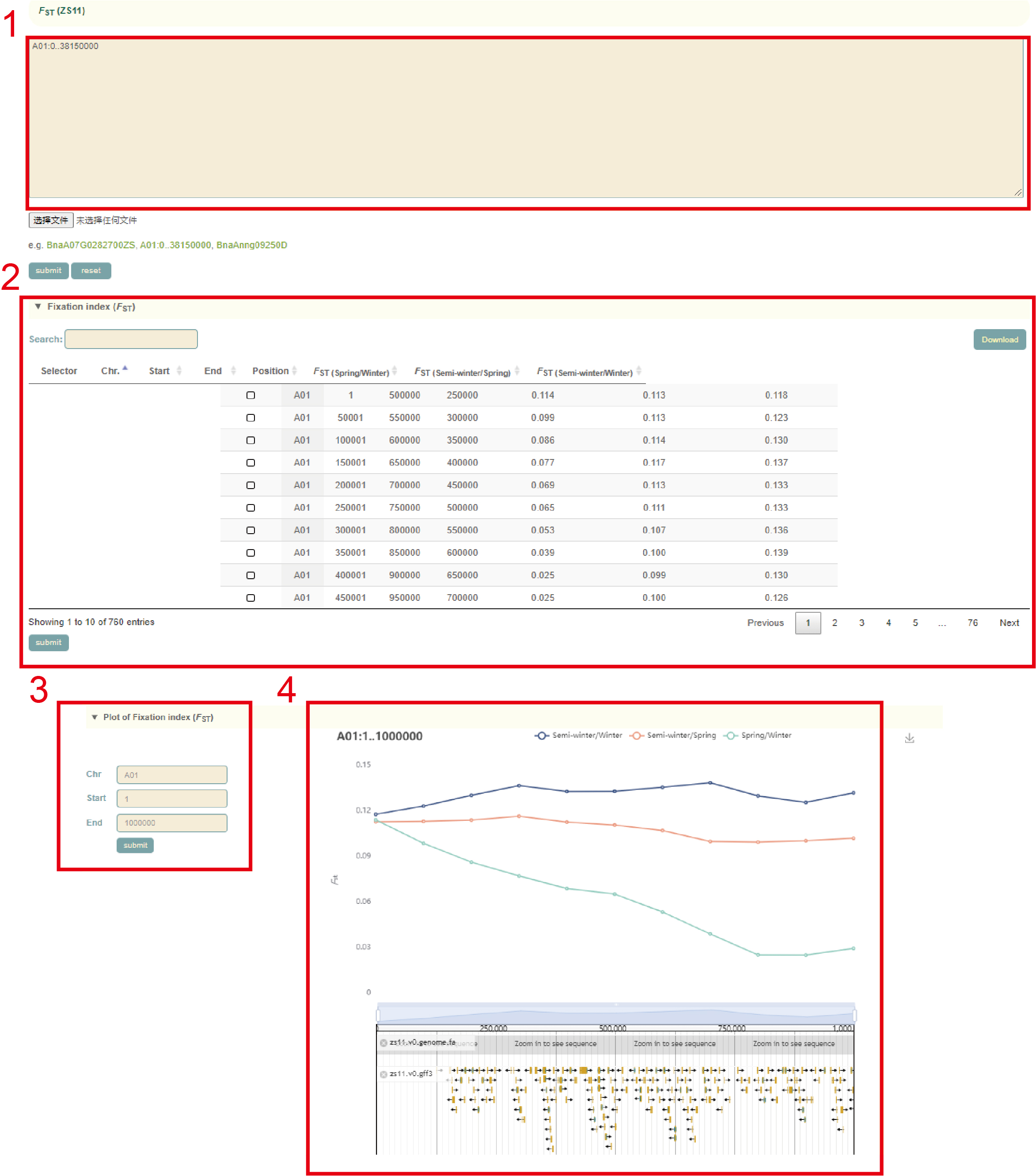
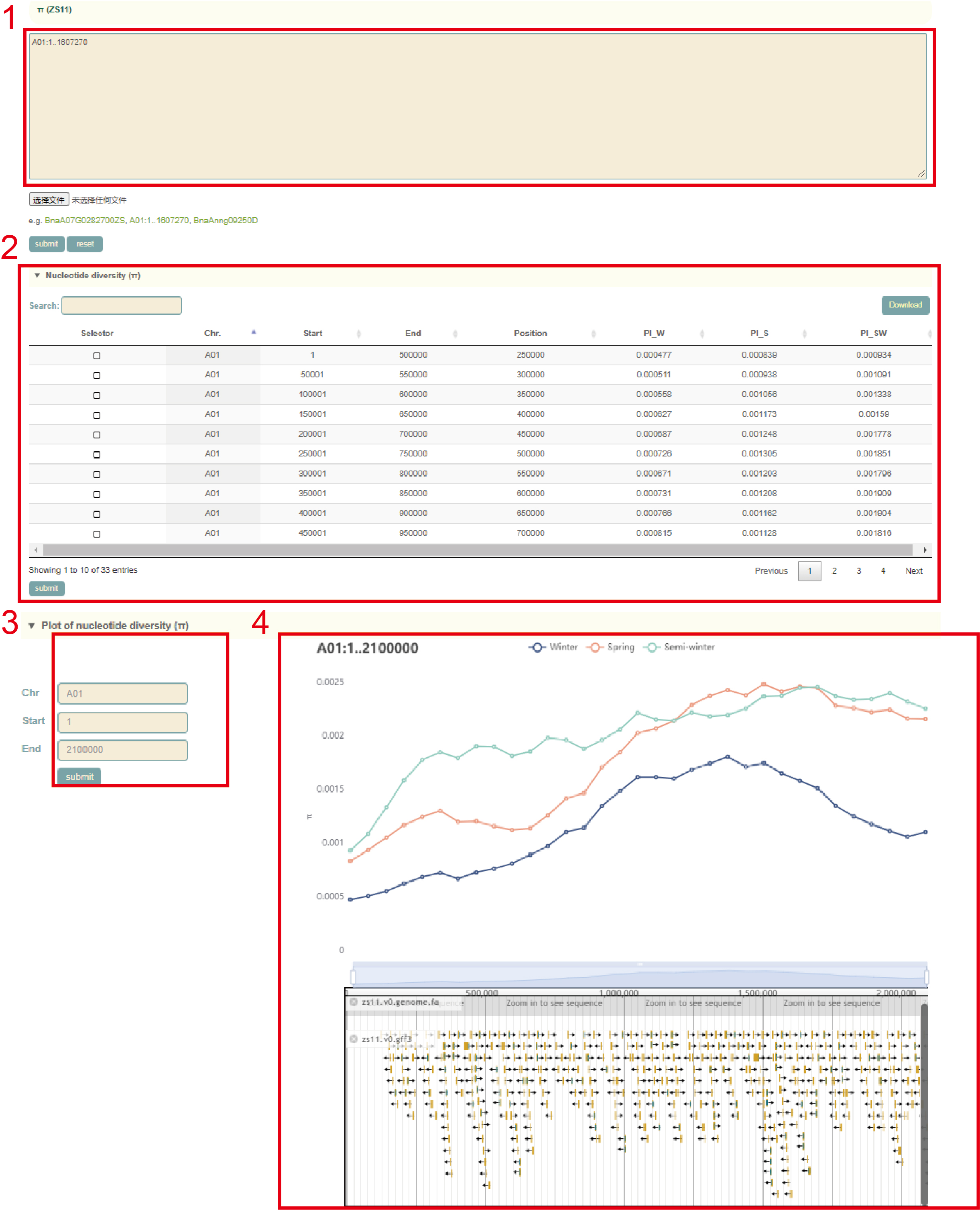
To identify genomic regions during the domestication and selection process, pairwise fixation statistic (FST), genetic diversity (π) and Ka/Ks values were calculated.
In the FST module, the user can submit the gene ID or genomic region in the search box(box 1), and then clicks "submit" to submit. Then, the FST values (box 2) and visualization results (box 3, box 4) of all windows (50 kb) in the area will be showed. The lines with different colors in the figure represent the FST values of the pairwise comparison between the three ecotypes. Users can also change this region on the left side of the page (box 3).
The usage of the Pi module is similar to that of FST. The user first submits the gene ID or genomic region (box 1) to query in the search box, and clicks "submit" to submit. Then, the Pi values (box 2) and visualization results (box 3, box 4) of all windows (50 kb) will be obtained. Users can also change this region on the left side of the page (box 3).
In the Ka/Ks module, the user first submits the gene ID or genomic region to query in the search box(box 1), and clicks "submit" to submit. The Ka, Ks, and Ka/Ks values (box 2) and visualization results (box 3, box 4) of the genes in this region are then obtained. Users can also search in the resubmission area on the left side of the page (box 3).
Variation
Single-locus module
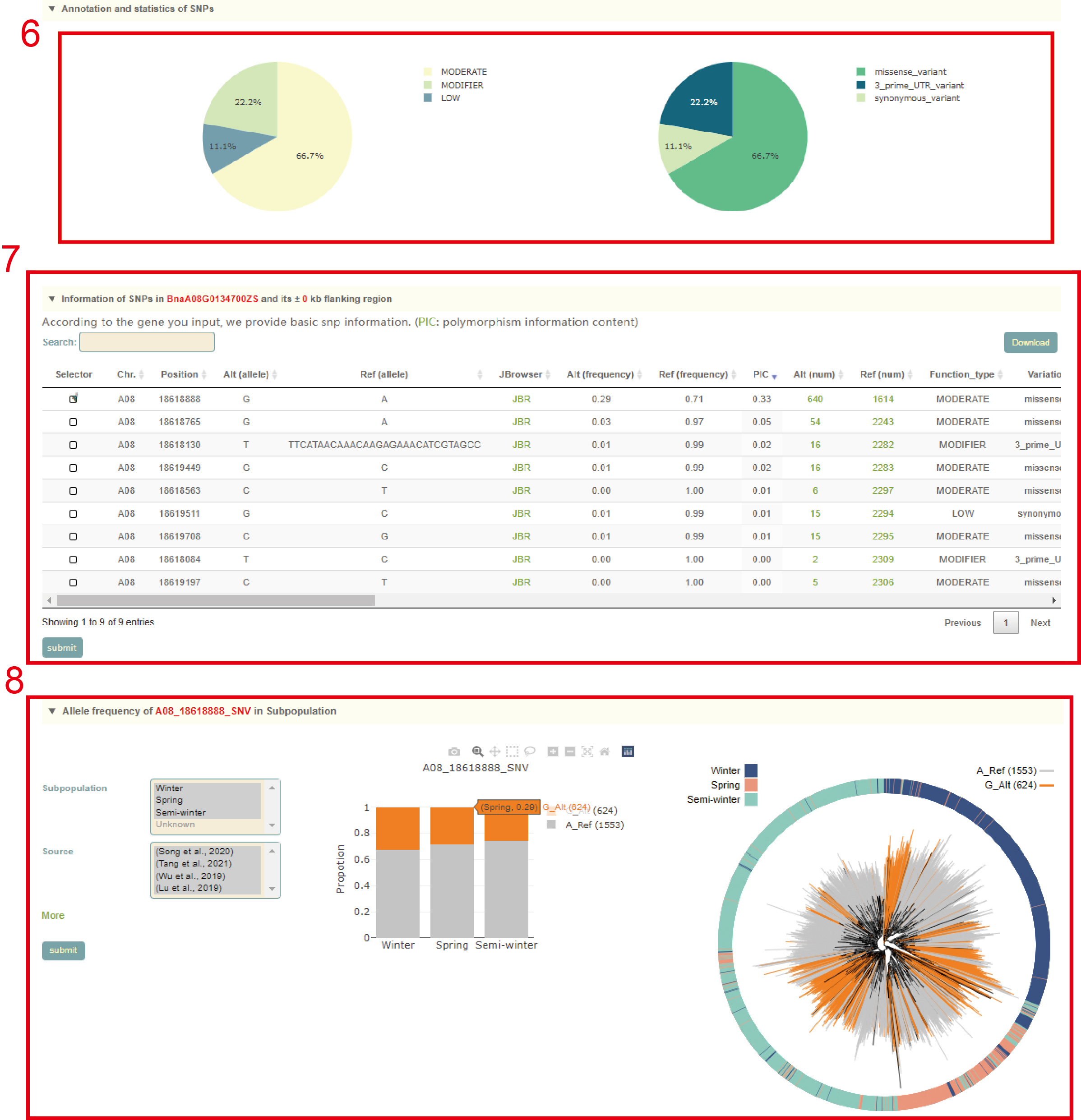
In the Single-locus module, users can search for genetic variation information in genes or genomic regions according to the gene ID, genomic region and gene index (box 1). The database integrated SNPs, InDels and SVs, and users can query by SNP or SV mode (box 2). In addition, users can also analyze the haplotypes composed of multiple SNPs in a gene through Haplotype mode, or perform combined analysis of SNPs and SVs using the merge mode (box 2). Take the search for the BnaA08.FAE1 (BnaA08G0134700ZS) gene as an example, the user enters "FAE1" in the Gene ID, then selects the "SNP Mode" (box 2), and then clicks 'submit' to query to obtain the related information.
The first page of the results is the statistics of the variation data of all homologous genes of the FAE1 gene in the ZS11 genome, such as the number of SNPs and SVs in the gene region (box 3). In box 3, users can click the radio box on the left side of the table to select one of the homologous genes of FAE1 gene, and then click the submit button to further analysis. By the way, users can also click the multi-selection box on the right side of the table to select multiple genes at the same time, and then click the 'Multi-locus model' button at the bottom right corner of the table to jump to the 'Multi-locus' module for subsequent analysis. Here, we take BnaA08.FAE1 (BnaA08G0134700ZS) gene as an example. After the user selects and submits the column of the gene in box 3, the relevant information will be displayed at the bottom of the table.
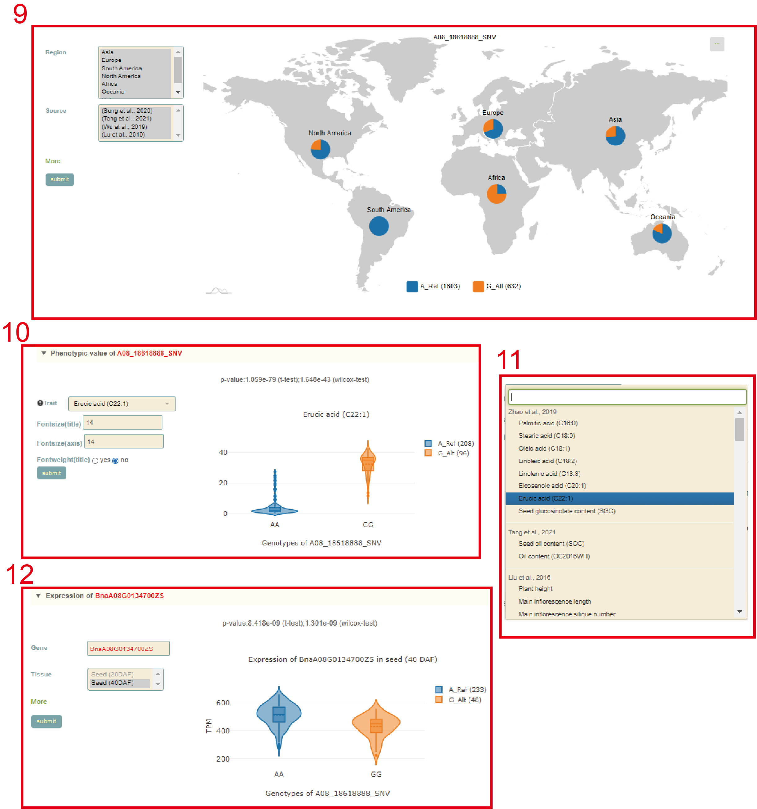
This is followed by a visualization of the distribution of variants in homologous genes, where different colored triangles represent variants with different variation effects. The user can move the mouse to the position of the corresponding mutation to view the specific information of the mutation (box 4). Then there is the BnaA08.FAE1 gene structure diagram, the user can move the mouse to the position of the corresponding variant and click to select the specific information to view the variant (box 5). Next, the user will get the statistics of the variants contained in the gene (box 6) and a list of all variants (box 7). The user can check the variant he wants to find in the first column. Then, based on the variant selected by the user, the page will give the frequency distribution of the variant in different subgroups (box 8) and the frequency distribution in the population in different geographic regions (box 9). Then, users can submit the phenotype to browse in the phenotype search bar to view the difference in phenotype values of accessions with different genotypes (box 10, box 11). Users can also submit the gene of interest in the gene search bar to view the difference in gene expression levels of accessions with different genotypes (box 12).

Multi-locus module
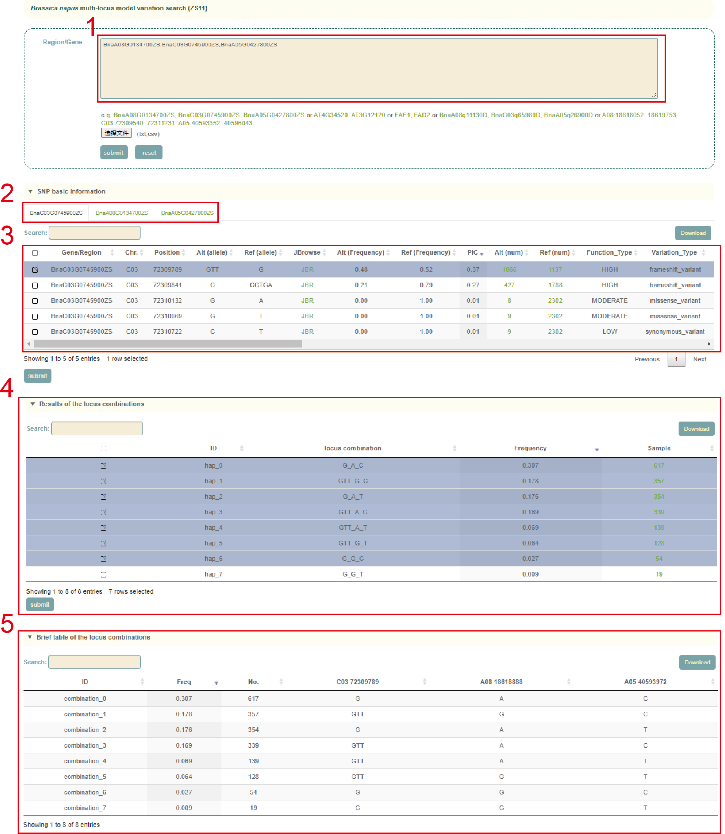
In the Multi-locus module, the user first entered the multiple gene IDs to query in the search box, and clicks 'submit' to submit (box 1). Next, as for the queried genes (box 2), the user selects the SNP ID to query and clicks 'submit' to submit (box 3). Then, the page will list the different haplotypes composed of these SNPs and haplotype frequencies (box 4). After users checked the haplotype they want to query in the first column, the page will list the sequence composition of the haplotype (box 5) based on the variants selected by the user. Then, the page will list the difference in phenotype values corresponding to accessions with different haplotypes(box 6). Users can also submit genes of interest in the gene search bar to view the differences in gene expression levels of accessions with the different haplotypes (box 7).

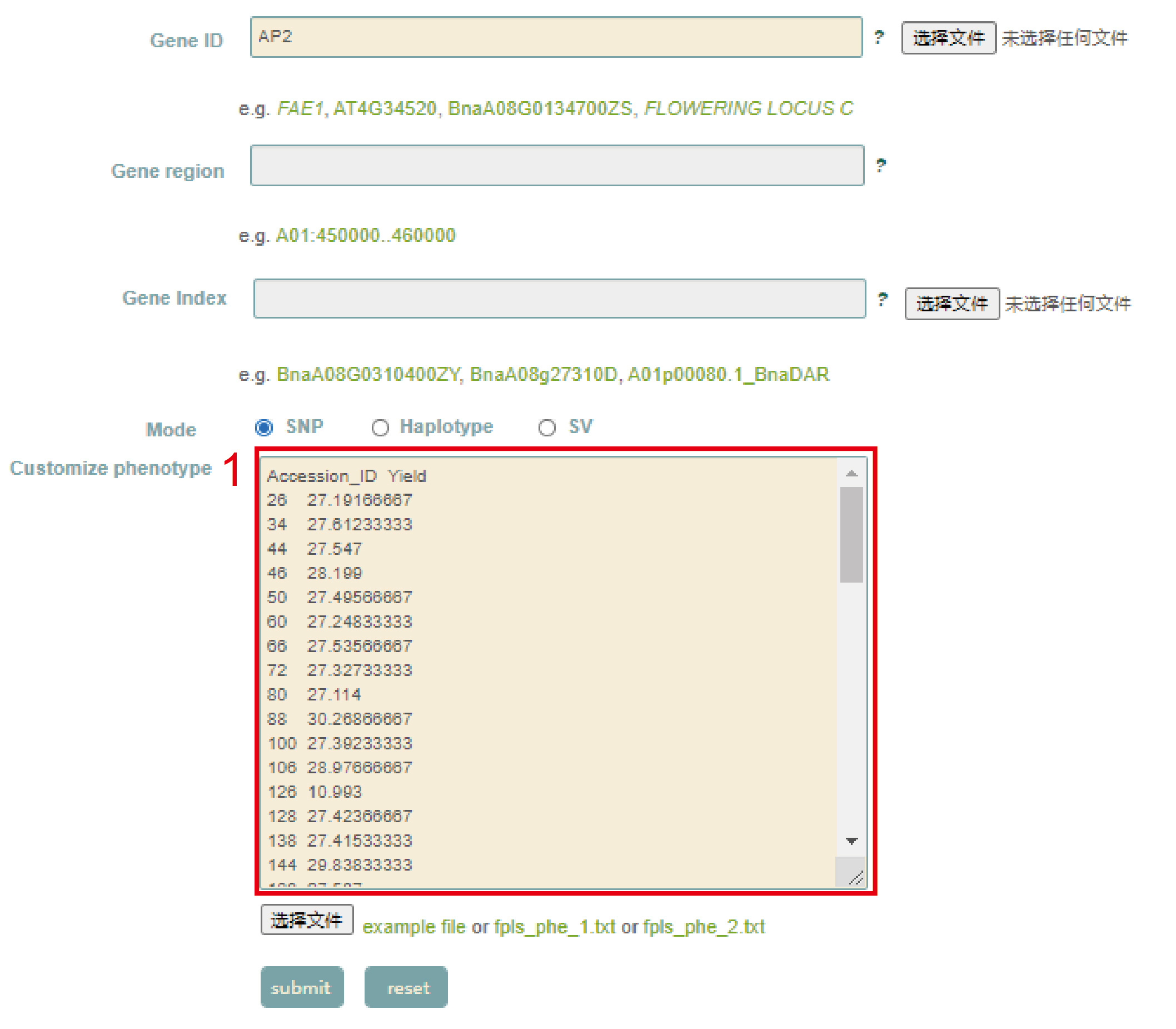
Customized phenotype association
In the Customized phenotype association module, users can directly paste the phenotype data (box 1) in Customize phenotype, or upload a local phenotypic data file, and then use it according to the operation mode of the Single-locus module.
Transcriptomics
Expression profile (ZS11 library)
Expression profile (ZS11 library) module can facilitate the identification of gene functions, which is greatly needed in rapeseed. Expression profile (ZS11 library) module contains gene expression levels from 91 libraries of ZS11 (Zhongshuang11), including covering eight different tissues covering 3 distinct developmental stages during its life cycle, including cotyledon, root, stem peel, leaf, bud, flower, silique, silique wall and seed. Especially, there exist 26 and 23 time points in seed and silique wall respectively and 24 leaf developmental time points, with 2 day intervals.
In this module, Users can search the expression level information of the gene of interest through three gene modes including gene ID, genome interval and gene index (box 1). For example, when the user enters FT, the information of the six homologous genes on the ZS11 genome will be obtained first in box 2, including the gene id of the corresponding Darmor genome, the corresponding Arabidopsis thaliana homologous gene ID and gene name, Physical location and functional descriptive information of genes. Then, the page will give data and visual displays of the expression levels of these genes in all libraries, such as heatmaps (box 3), table (box 4), line graphs (box 5), and boxplots (box 6). Then, in box 7, the statistical information of gene expression level is obtained, including how many libraries it is expressed in, the mean, median, maximum, minimum, standard deviation and coefficient of variation of the expression.
.jpg)
Expression profile (meta library)
We collected gene expression profiles of 2,791 published RNA-seq libraries. Similar to Expression profile (ZS11 library), this module also supports three search modes: gene ID, genome interval and gene index (box 1). For example, when the user enters FT, the statistical information of the expression level of the gene is obtained, including how many of the 2,791 libraries are expressed, the mean, median, maximum, minimum, standard deviation and coefficient of variation in the "Summary of gene expression" (box 2). At the same time, the information on the 6 homologous genes on the ZS11 genome will be obtained first in the "Basic information of genes" (box 4), including the gene id of the corresponding Darmor genome, the corresponding Arabidopsis homologous gene ID and gene name, the physical location and functional description of the gene. In box 4, users can click the radio box on the left side of the table to select one of the homologous genes of FT, and then click the submit button to further analysis. Here, we take BnaA02G0156900ZS gene as an example. After the user selects and submits the column of the gene in box 4, the relevant information will be displayed at the bottom of the table. Box 5 will show the data and visualization of the expression levels of BnaA02G0156900ZS in all libraries. In box 8, the user will get the expression of these genes in different ecotypes of rapeseed during the vernalization process and double-low and double-high rapeseed, and the user can know whether these genes are related to the breeding improvement process according to the difference in gene expression between accessions. In addition, we also provide a comparison of gene expression levels among heterosis accessions in groups, so that users can understand whether these genes are related to heterosis (box 9).
.jpg)
Population expression
We integrated the gene expression data of 700 samples of seeds and leaves at 20 days after flowering, 40 days after flowering.
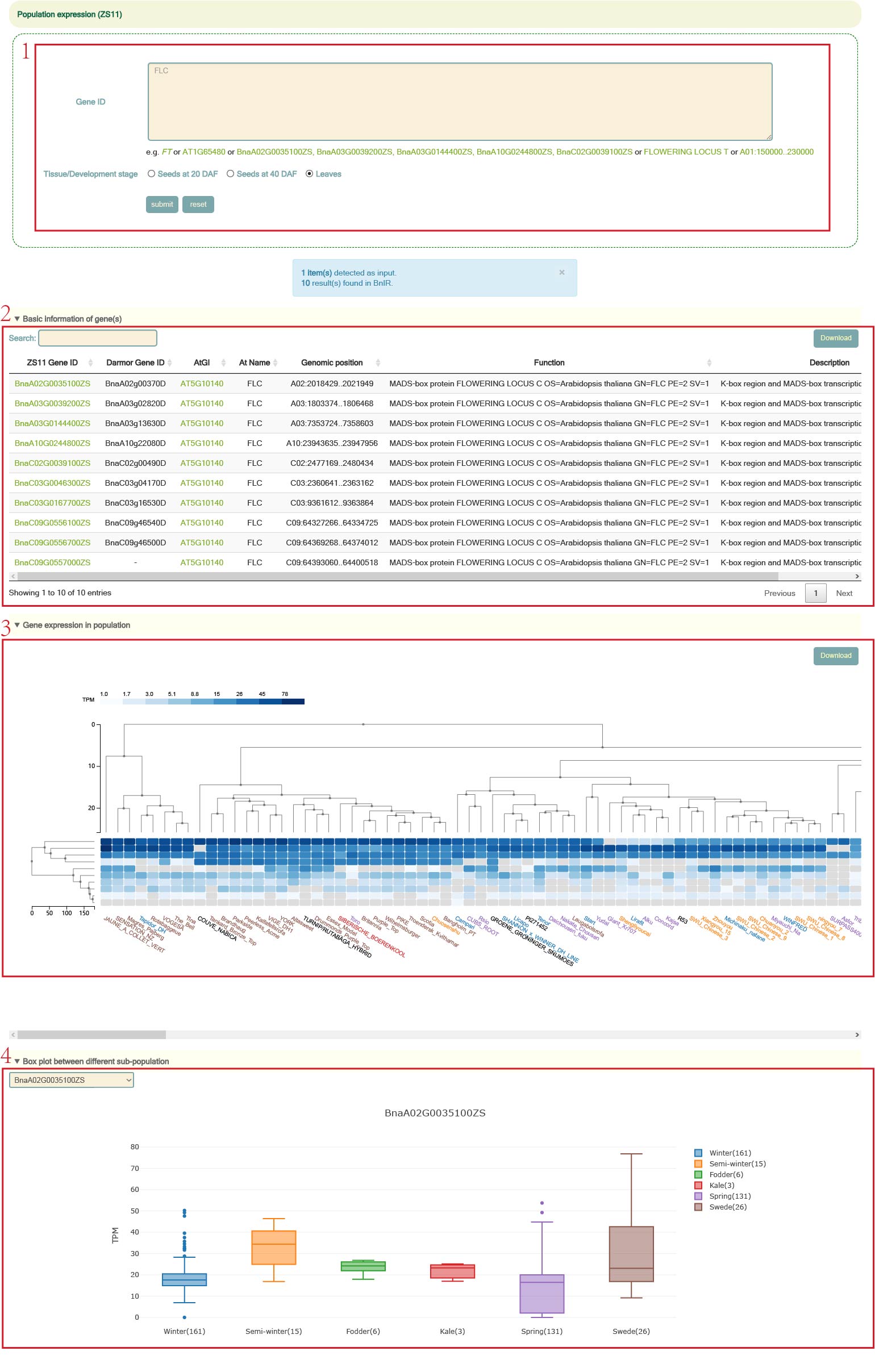
The user can enter the Arabidopsis gene ID, B. napus gene list or genomic region, and then select the tissue to query the expression level of the gene of interest (box 1). For example, when the user enters FLC and selects "Leaves", the following result can be obtained. "Basic information of genes" (box 2) is the 10 homologous gene information on the ZS11 genome, including the gene id of the corresponding Darmor genome, the corresponding Arabidopsis homologous gene ID and gene name, and the physical location of the gene and functional description information. Then there are the clustering results of the expression levels of these genes in the population, and the texts in different colors on the horizontal axis represent rapeseed of different ecotypes (box 3). Finally, boxplots of gene expression levels of different ecotypes of B. napus can be viewed (box 4).
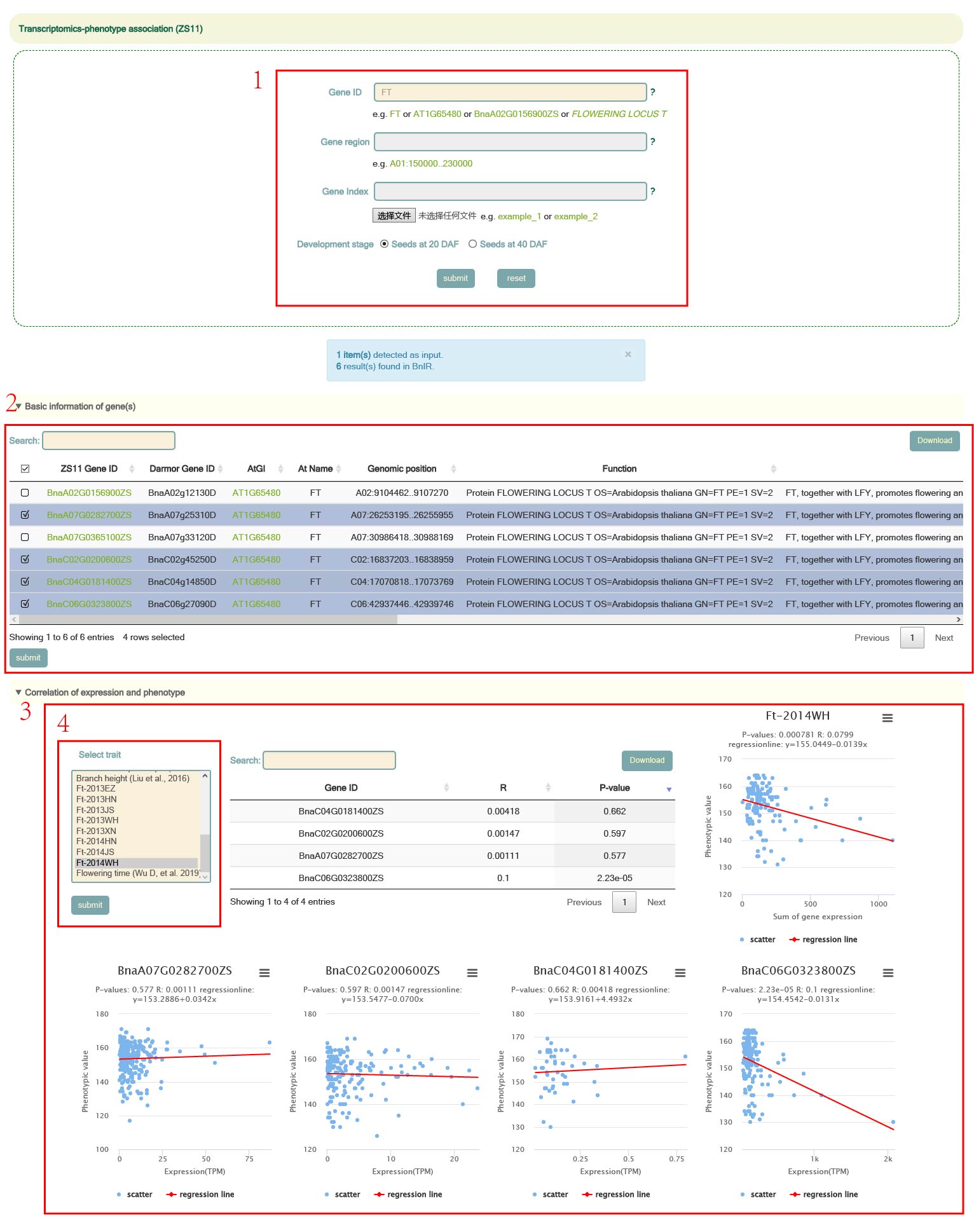
Transcriptomics-phenotype association
In the Transcriptomics-phenotype association module, we integrated data from seeds at 20 days after flowering, 40 days after flowering, and 20 phenotypes. Users can enter Arabidopsis gene ID, B. napus gene list or genomic region, and then select tissue to query the correlation between the expression level of the gene of interest and these phenotypes (box 1). When the user enters a gene ID and selects a tissue and clicks 'submit' to submit, "Basic information of genes" will give information on the homologous genes on the ZS11 genome (box 2). Then, by selecting the phenotype and clicking 'submit' (box 3), users can obtain the correlation information of these genes and phenotypes and the scatter plot of genes and phenotypes in the "Expression-phenotype basic information" category (box 4).
eFP(single gene module)
Electronic Fluorescent Pictographic (eFP) provides a suit of interactive tools, allowing users to comprehensively view gene expression levels among 8 tissues at different stages of development. By entering "Data Source","Mode","Primary Gene ID","Secondary Gene ID","Signal Threshold" and clicking "Go",you will see the specific expression of genes in various tissues under controlled conditions. User can select one data source from 'Tissue', 'Hormone' and 'Adversity' (box 1), one mode from 'Absolute', 'Relative' and 'Compare' (box 2) and Gene ID (box 3). Then, the eFP figure of gene expression will be obtained (box 4). Users can move the mouse over the tissue in the figure to query the gene expression value.
The following is a detailed explanation of three modes in eFP:
Absolute: The absolute expression level for a given gene.

Relative: The relative expression of any given gene is compared to a control data (the median expression value of that gene for all samples that were measured), which can be used to study where the gene is most-prominently expressed.

Compare: The relative expression of any given gene (primary gene) can be compared to any other gene (secondary gene). Normally, the genes that are constitutively expressed in all tissues (housekeeping genes) are used as the secondary gene.
.jpg)
eFP(multiple gene module)
Similar to eFP(Single gene Module), eFP(Multiple gene Module) provides an eFP browser with multiple gene expressions. In this module, the user can view the sum of the expression levels of these homologous genes by entering the Arabidopsis gene ID to obtain the gene name in the eFP browser.
Phenotype
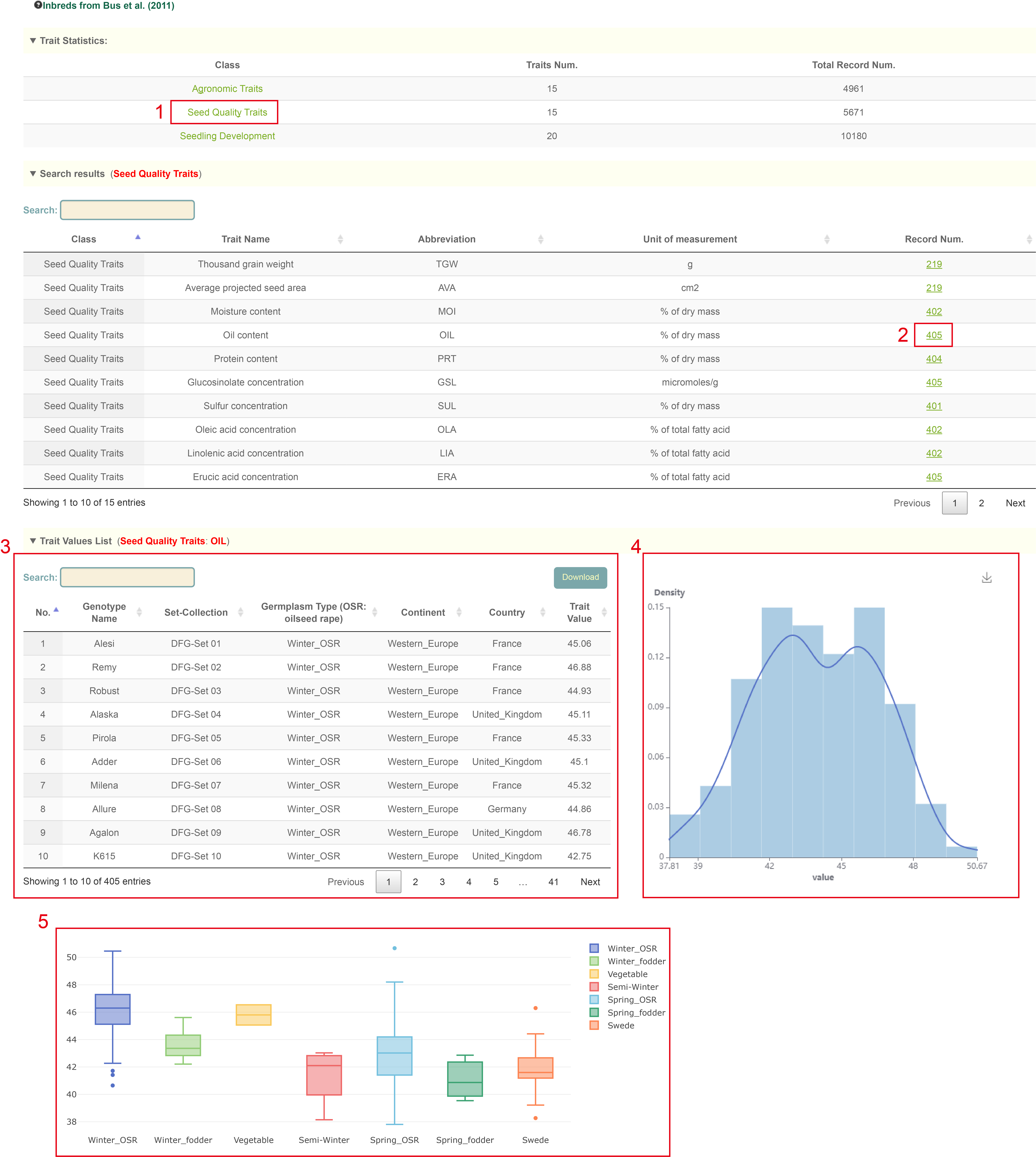
In Phenotype portal, we collected 118 traits of 2,512 accessions, including 50 traits of 525 inbred lines, 36 glucosinolate related traits of 288 accessions, five traits of 991 accessions, three flowering time traits of 210 accessions and 27 traits of 505 accessions. These phenotypic data are grouped into five modules based on their data sources, and users can browse these phenotypic datasets in the corresponding modules. Taking 522 Inbred Lines (Bus et al. 2011) as an example[2], clicking on 522 Inbred Lines (Bus et al. 2011) takes you to the phenotypic page of that population. The first is categorical statistics of all types of phenotypes. For example, if users want to search the oil content, users can click "Seed Quality Traits" (box 1) to obtain 15 seed quality-related phenotypes, including oil content phenotype data of 405 accessions. Then click '405' (box 2) to obtain the specific phenotypic value information of 405 samples (box 3), the histogram of phenotypic value distribution (box 4) and the boxplot of phenotypic value of different rape types (box 5).
Epigenetics
Histone modification
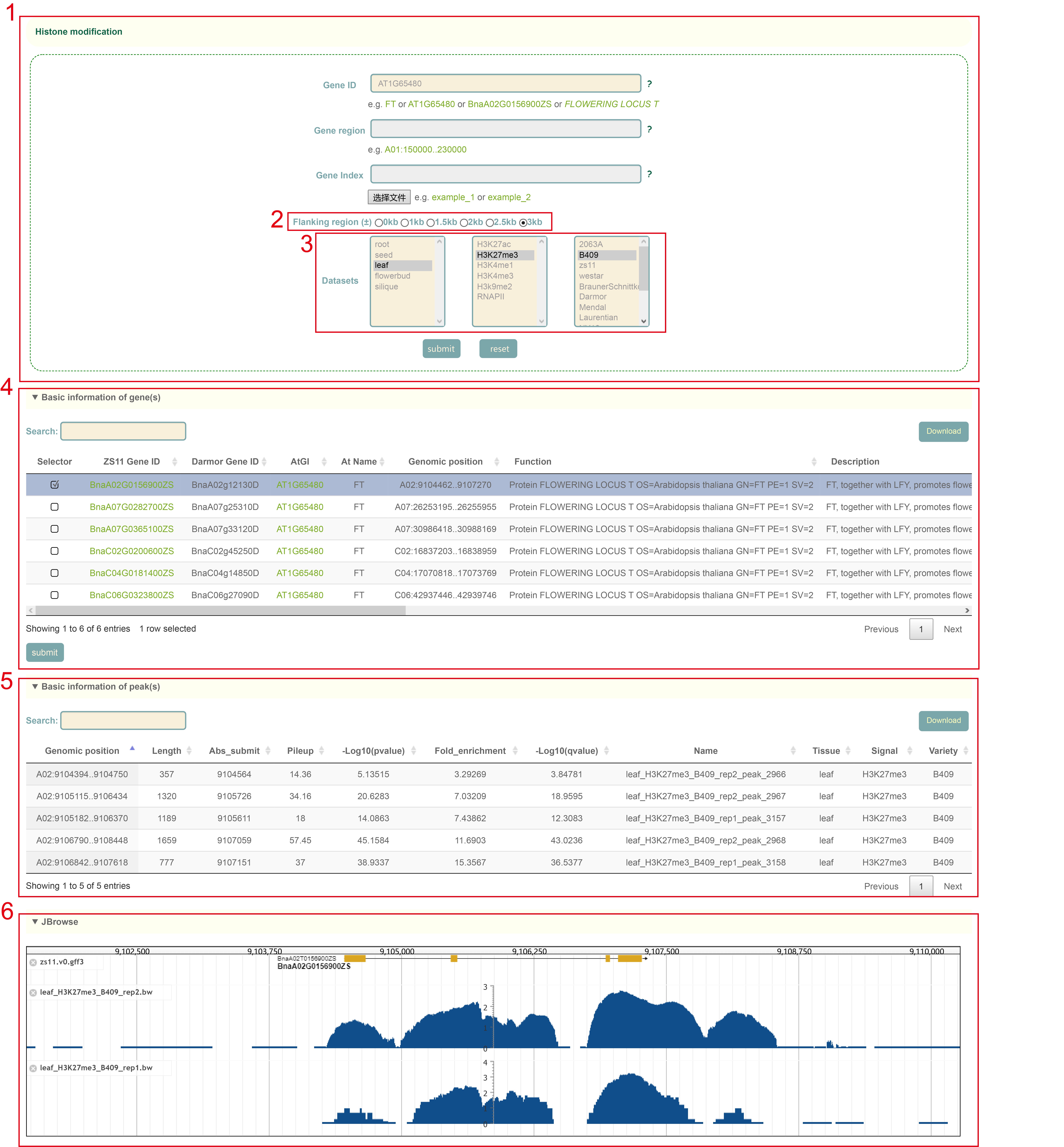
The user first enters the gene ID to query (box 1), the genomic region, histone modification type, accession and tissue. Take AT1G65480 as an example, first enter AT1G65480 in Gene ID, and choose the 3kb in Flanking region (box 2), then select tissue, histone modification type and accession in Datasets (box 3), and then click 'submit' to submit. In the Results section, the physical location and functional annotation information of the homologous genes of AT1G65480 in the ZS11 genome are listed first (box 4). Then there is the peak information in this region (box 5). The last is the coverage of reads in this region in the Jbrowser browser (box 6).
DNA methylation
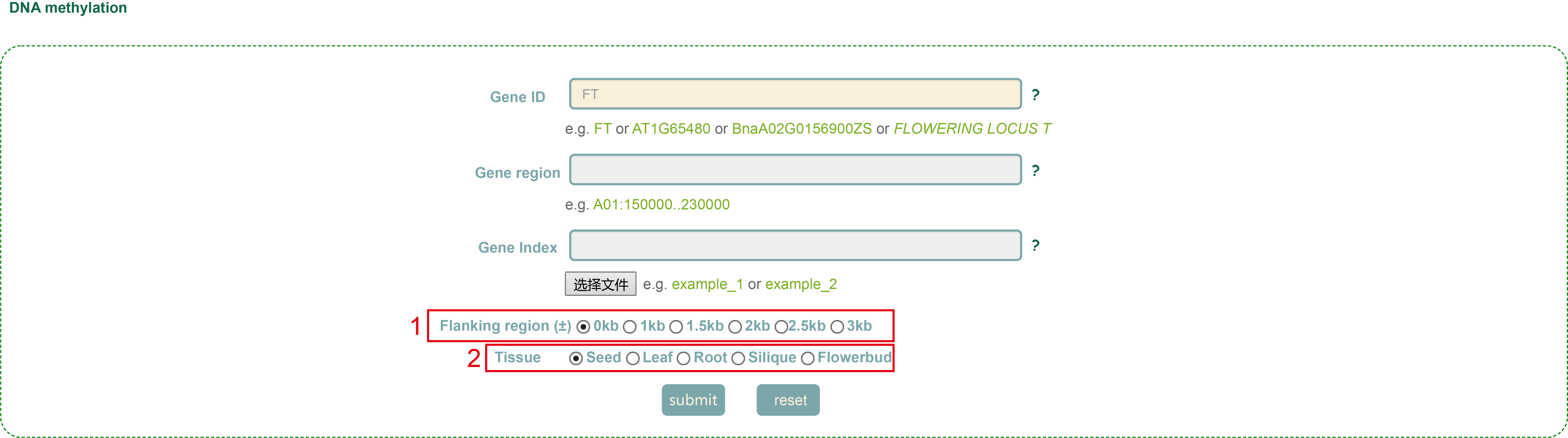
In the DNA methylation module, we integrated data from 54 WGBS-seq libraries and calculated the methylation ratio of each gene region in each library. Users can enter the gene id or genomic region, then set the region size (box 1) in Flanking region, select Tissue (box 2), and click 'submit' to query.
Chromatin accessibility
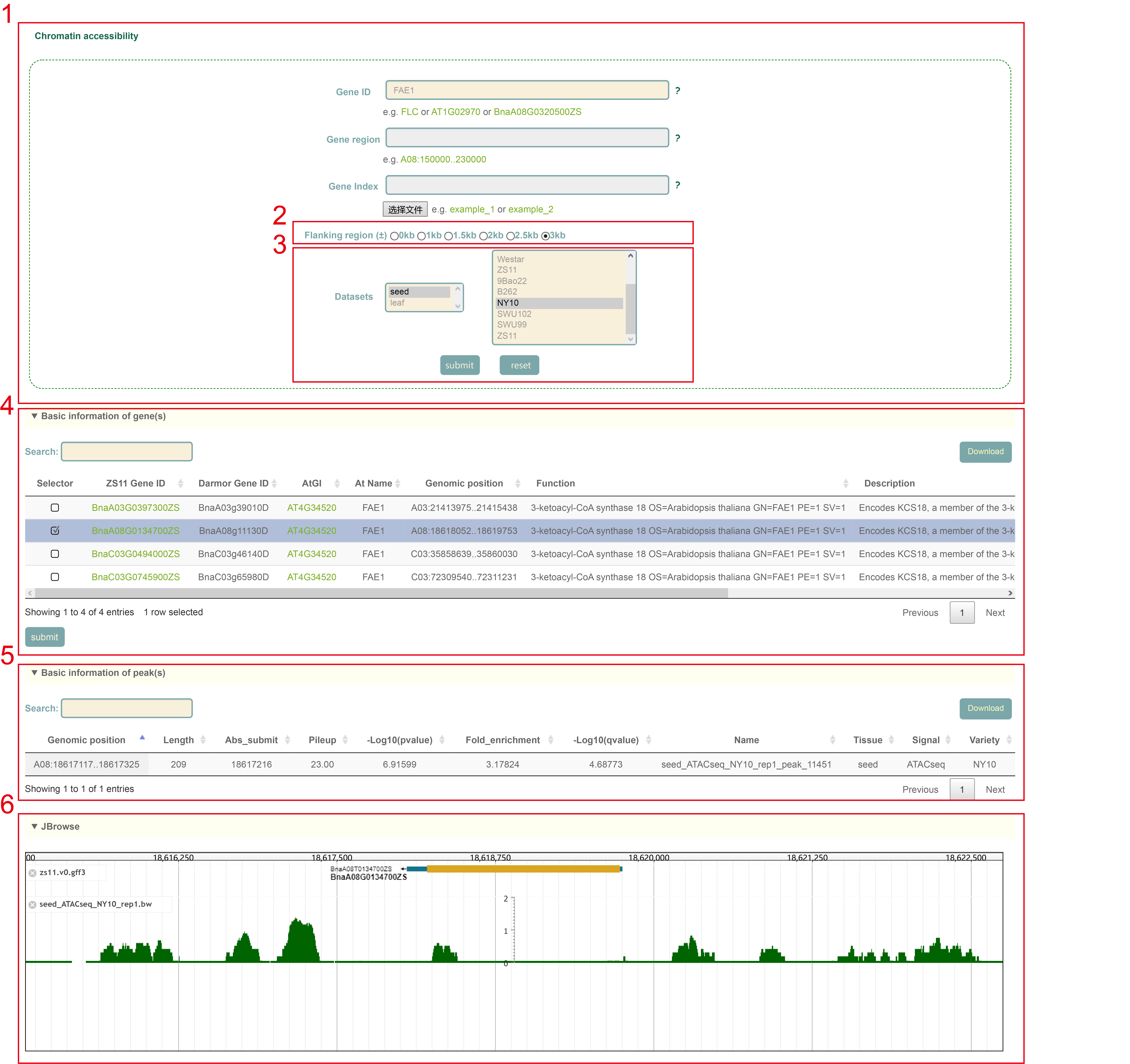
The user first enters the gene to query (box 1), the genomic region, histone modification type, the sample and the tissue. Take FAE1 as an example, first enter FAE1 in Gene ID, set a 3kb surrounding area in Flanking region (box 2), then select tissue and sample in Datasets (box 3), click 'submit', or chromatin accessibility values for the 3kb region surrounding this gene. In the Results section, the physical location and functional annotation information of FAE1 homologous genes in the ZS11 genome are first listed (box 4). Then the peak information is listed (box 5). The last is the coverage of reads in this region in the Jbrowser browser (box 6).
Chromatin interaction
In Chromatin interaction module, we collected and analyzed the Hi-C data of the three published accessions and obtained their chromatin interaction features.
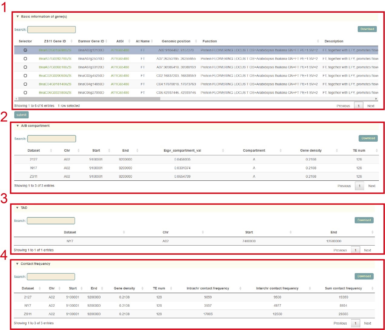
Firstly, the user enters the gene, genomic region or gene index to query, or uploads the gene index file. Then clicks "submit" to submit. Next, the user will get the information list of the queried genes. The user can select the gene to be query by checking the first column (box 1) and click "submit" to submit. The user will then get the results of three parts including the A/B compartment (box 2), the TAD (box 3), and the chromatin interaction frequency for each 100kb region (box 4). Users can click "Download" in the upper right to download.

Multi-omics
GWAS
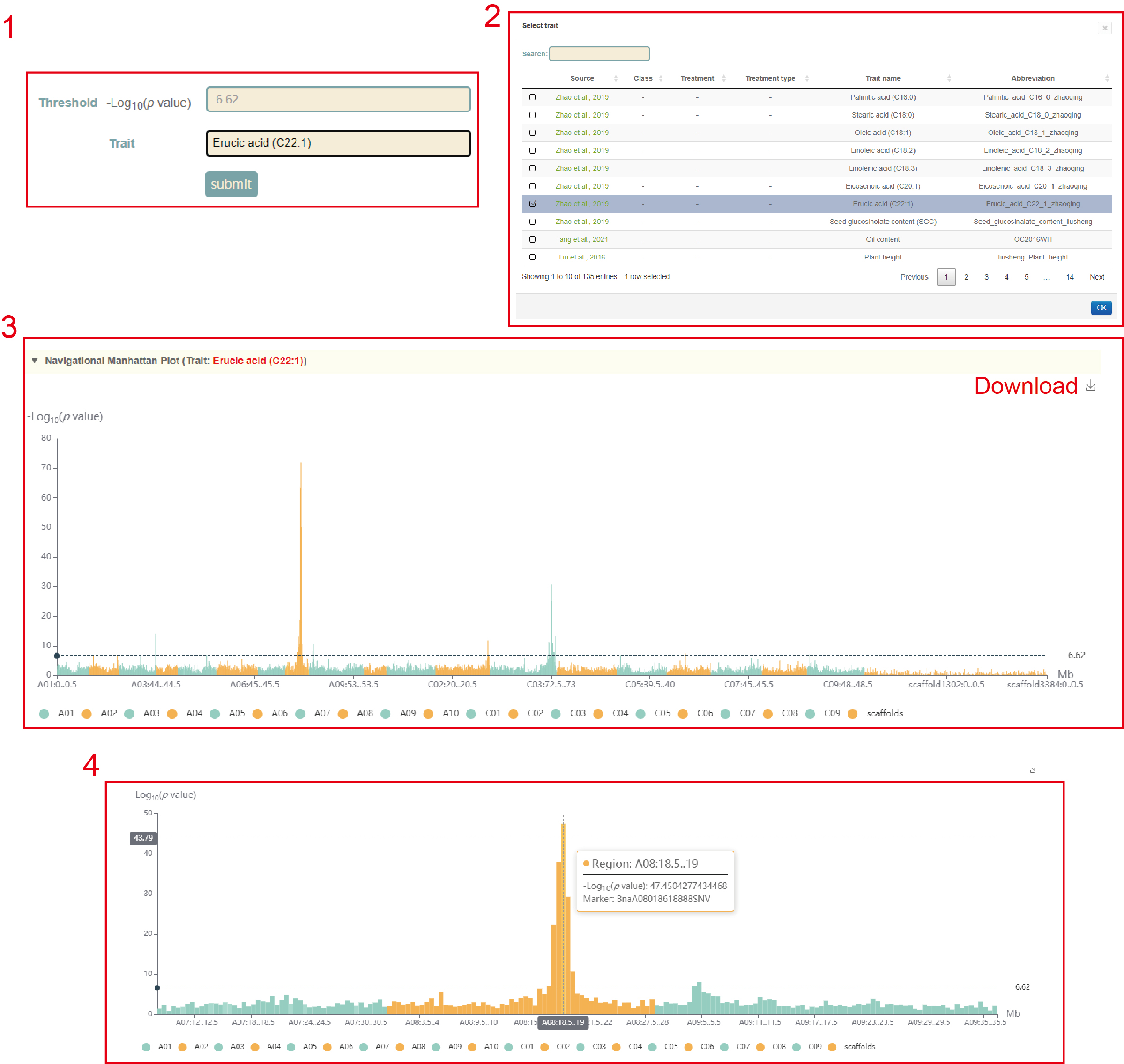
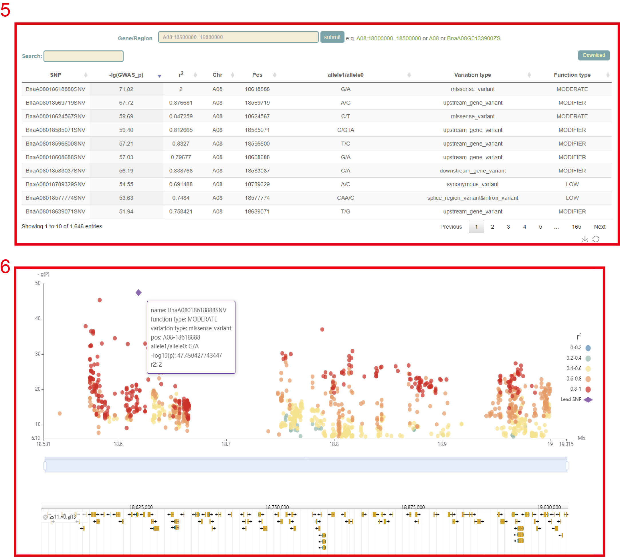
In GWAS module, the user firstly clicked the phenotype name(box 1), and then a dialog box for the phenotype list will pop up. The user selects the phenotype by checking the first column, then clicks 'OK', and then clicks 'submit', that is GWAS results for this phenotype can be viewed. The first is a manhattan plot (box 3) of a 500kb window, in which we denote the p-value of each window by the p-value of the most significant SNP in it. Here, the user can zoom in or out by sliding the mouse wheel, and then move the mouse to the corresponding window to browse the lead SNP and the corresponding p-value (box 4) in the window. The user can then click on the bars of this window to view all the significant SNPs within this region along with the corresponding GWAS statistics (box 5) and Manhattan plots (box 6).
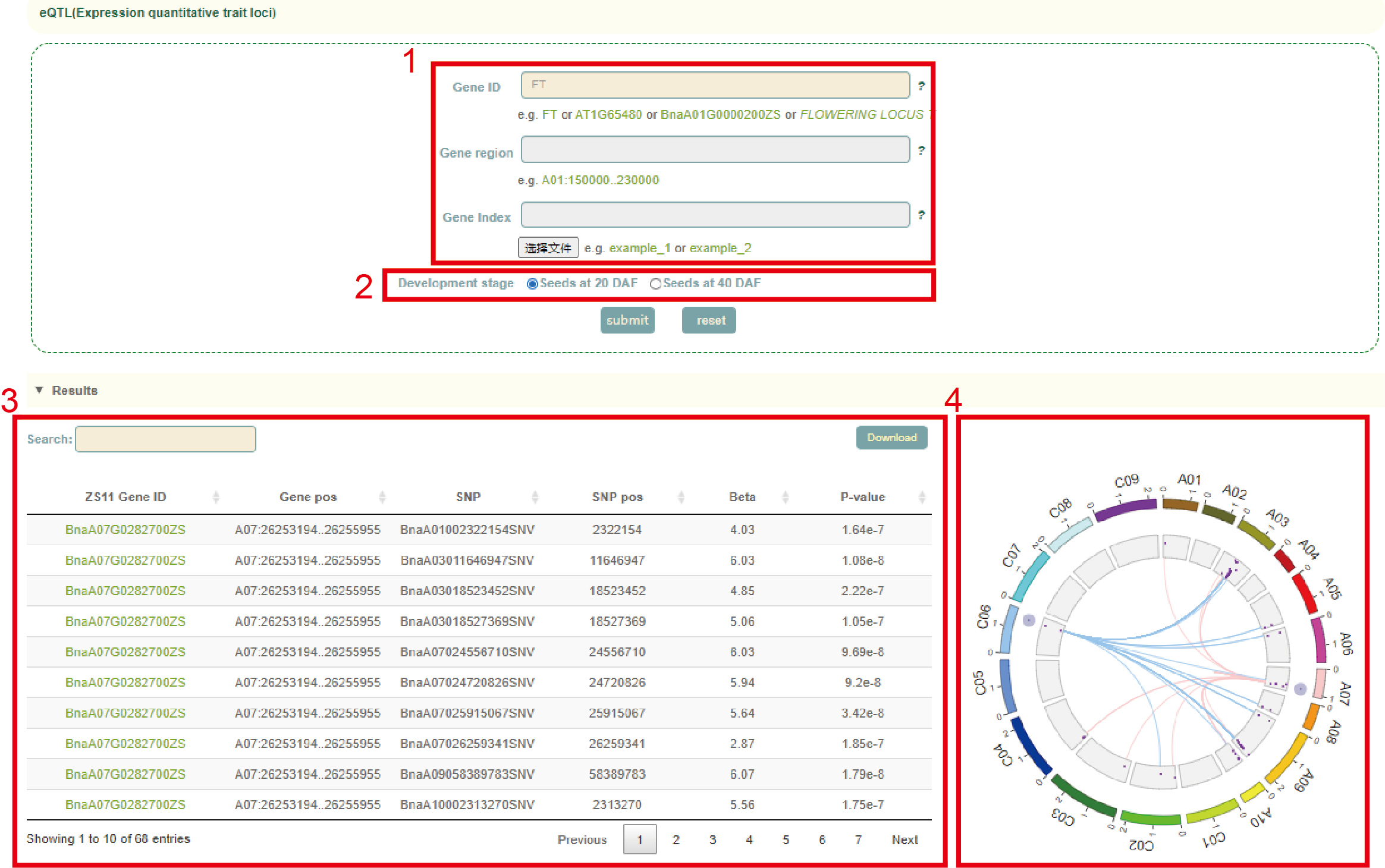
eQTL
In eQTL module, the user first searches for genes by gene ID(box 1), genomic region or gene index, then selects the tissue in the "Development stage", and clicks "submit" to submit. In the results, the first is a list of all SNPs significantly associated with the expression of this gene and the corresponding statistics, including beta and P-value (box 3). Finally, a circos diagram of the relationship between SNP and gene regulation was shown. Users can move the mouse to the corresponding point in the diagram to view the value of the statistic corresponding to 'eSNP-eGene' (box 4).
TWAS
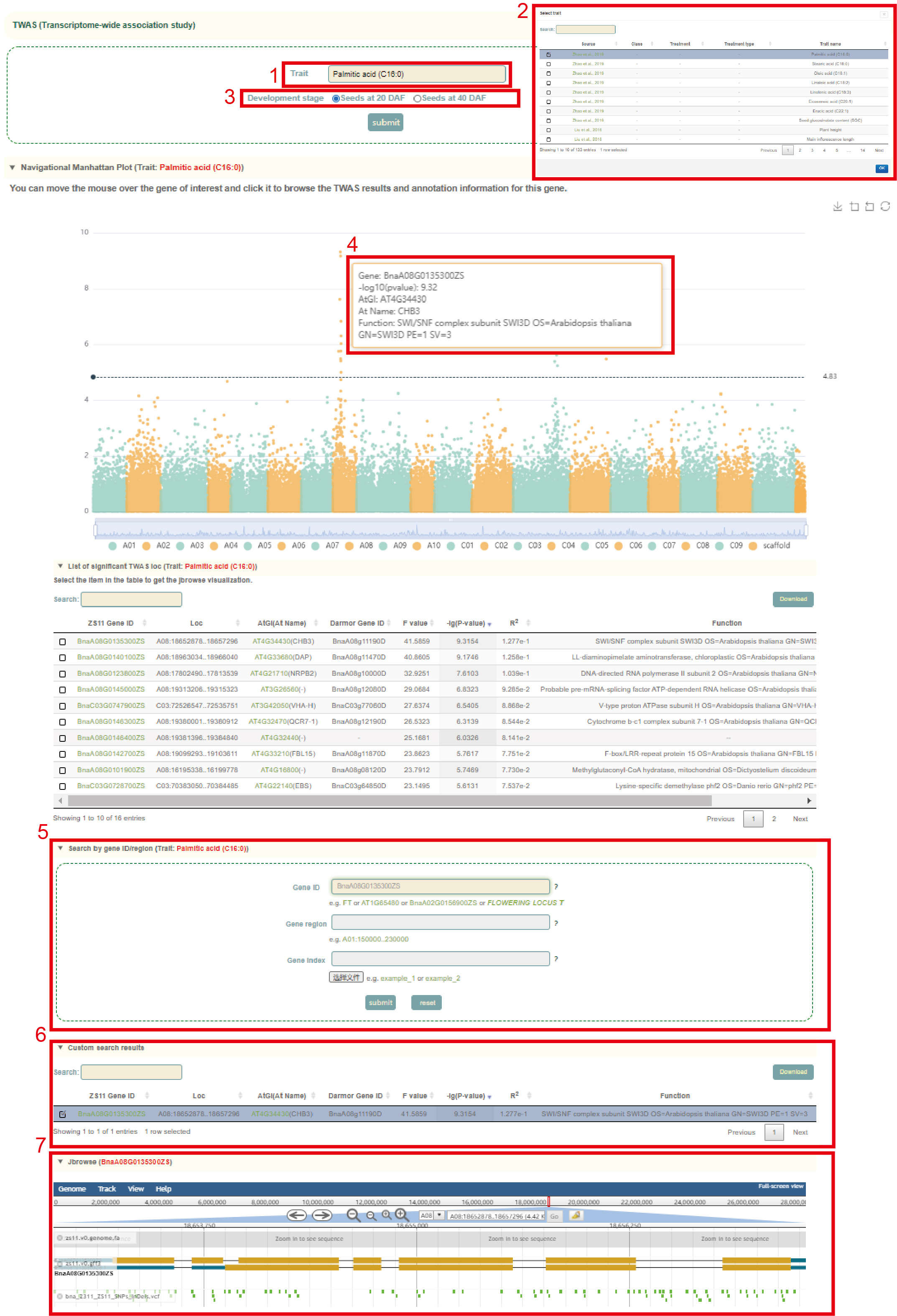
In the TWAS module, the user firstly clicked the phenotype name (box 1), and a dialog box for the phenotype list will pop up. The user selects the phenotype by checking the first column, then clicks 'OK', and then selects the corresponding organization (box 2), click 'submit' to view the TWAS results of the phenotype of the tissue. The first is a genome-wide Manhattan plot of all gene TWAS (box 3). Users can zoom in or out by sliding the mouse wheel, and then move the mouse to the corresponding point to browse the TWAS statistics of the gene (box 4). The user can then click on the corresponding point to view the TWAS statistics for this gene (box 6). Users can also search for genes by Gene ID, genome interval or Gene index (box 5) to view the TWAS results of these genes and browse the structure of these genes and the distribution of genetic variation near them in the Jbowser browser (box 7).
SMR
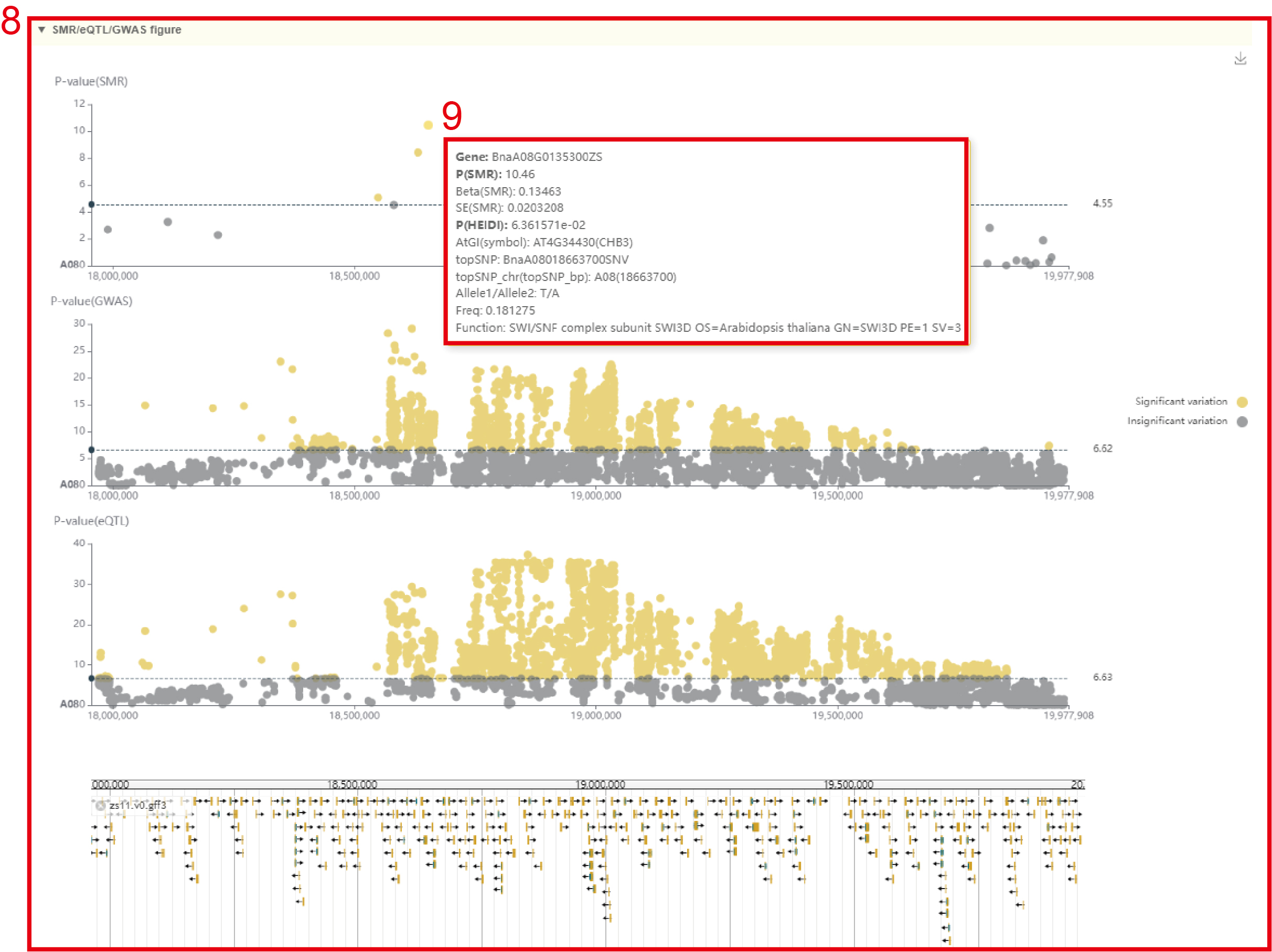
In the SMR module, the user chooses to click the phenotype name in box 1, and then a dialog box for the phenotype list (box 2) will pop up. The user selects the phenotype by checking the first column, then clicks 'OK', and then selects the corresponding tissue (box 3), click 'submit' to view the SMR results of the phenotype of that tissue. The first is a Manhattan plot of the SMR of all genes in the whole genome (box 4) and the information list of all significant genes (box 5). The SMR significance threshold is: P(SMR)<1 /n (20DAF: n=35,633, 40DAF: n=38,747), P(HEIDI test)>1.57*10-3. Users can zoom in or out by sliding the mouse wheel, and then move the mouse to the corresponding point to browse the GWAS, eQTL and SMR statistics of the gene (box 4). The user can then click on the corresponding point to view detailed statistics of the SMR for this gene (box 7). Users can also search for genes (box 6) by Gene ID, genomic region, or gene index to view SMR results of these genes. Next, the page gives the local Manhattan map of SMR, GWAS, and eQTL in the 1Mb region near the gene (box 8). Users can move the mouse to these points to view the corresponding SNP/Gene statistics (box 9). Finally, users can browse the structure of these genes and the distribution of genetic variation in their vicinity in the Jbowser browser.

Colocalization analysis
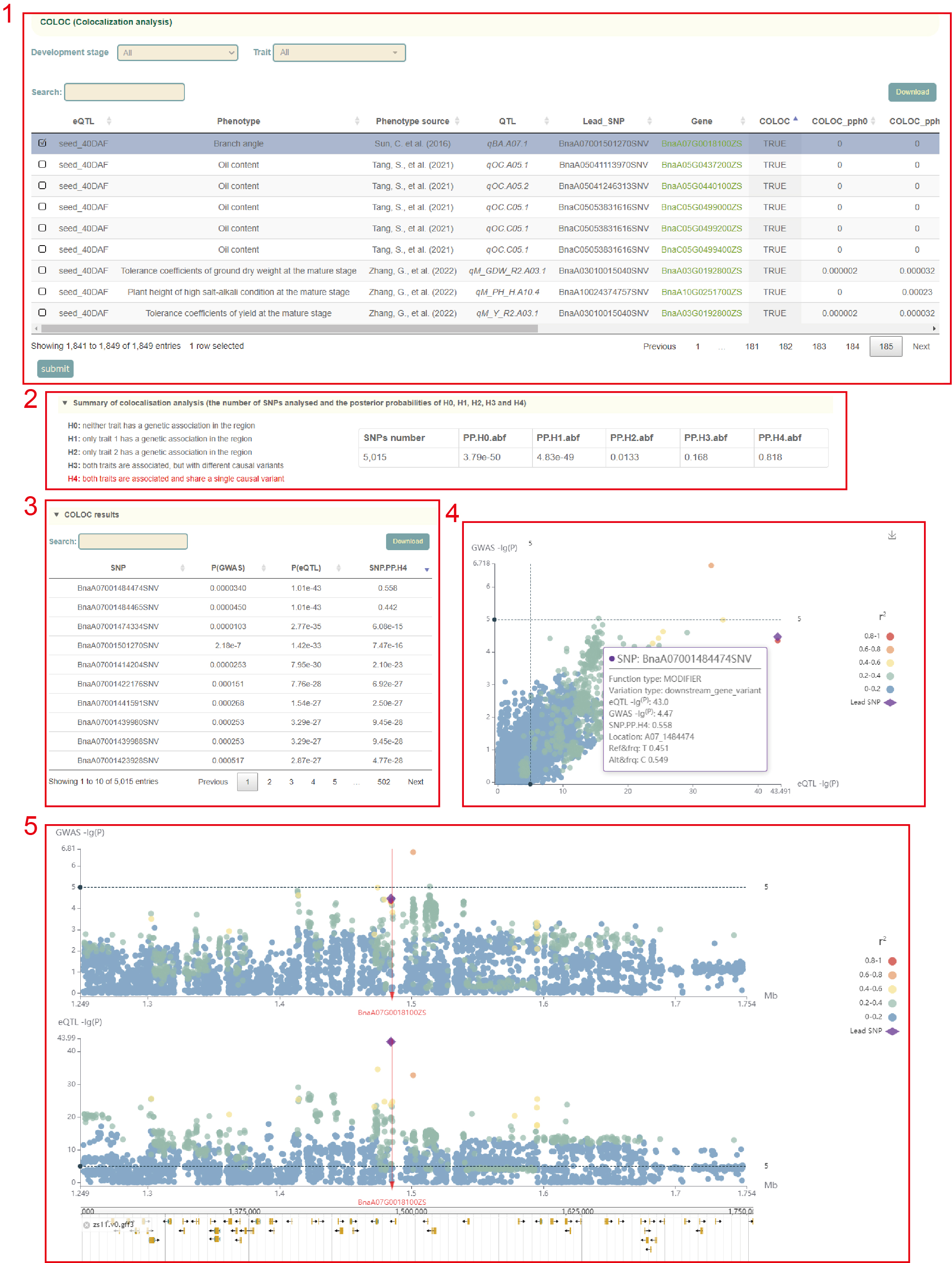
Based on the GWAS and eQTL results, we identified 1,849 associations between expressed genes with eQTL and GWAS loci by co-localization analysis. A total of 217 associations were identified by co-localization analysis, which were integrated into Colocalization analysis module.
In this module, the first part is a list of colocalization analysis results of eQTL and GWAS loci of 1,849 pairs of expressed genes (box 1), including all statistics of colocalization analysis, such as PPH0, PPH1, PPH2, PPH3, PPH4. Users can filter these results by selecting the tissue and phenotype by pulling down the Development stage and Trait menus. Then, the user can select the co-localization analysis results of the QTL and eQTL to be viewed next by checking the first column, and click 'submit' to submit. The results start with the main statistics of the results of the co-localization analysis of QTL and eQTL. The red text on the left represents the accepted hypothesis. If the PPH4 value is the largest among all PPH values, the text of the PPH4 hypothesis is marked in red, indicating to accept H4, which is "both traits are associated and share a single causal variant". On the premise of accepting H4, the P-values of GWAS and eQTL and PPH4 values of all variants in this region are listed(box 3), which can be used to locate the causal variation. And users can move the mouse to the figure to browse the detailed statistics of these variants(box 4). Then comes the visualization of the local Manhattan plot of the GWAS and eQTL in the region, and the user can also move the mouse over the points in the plot to see detailed statistics of these variants (box 5). Finally, users can browse the distribution of genetic variation near the gene in the Jbowser browser.
Metabolome
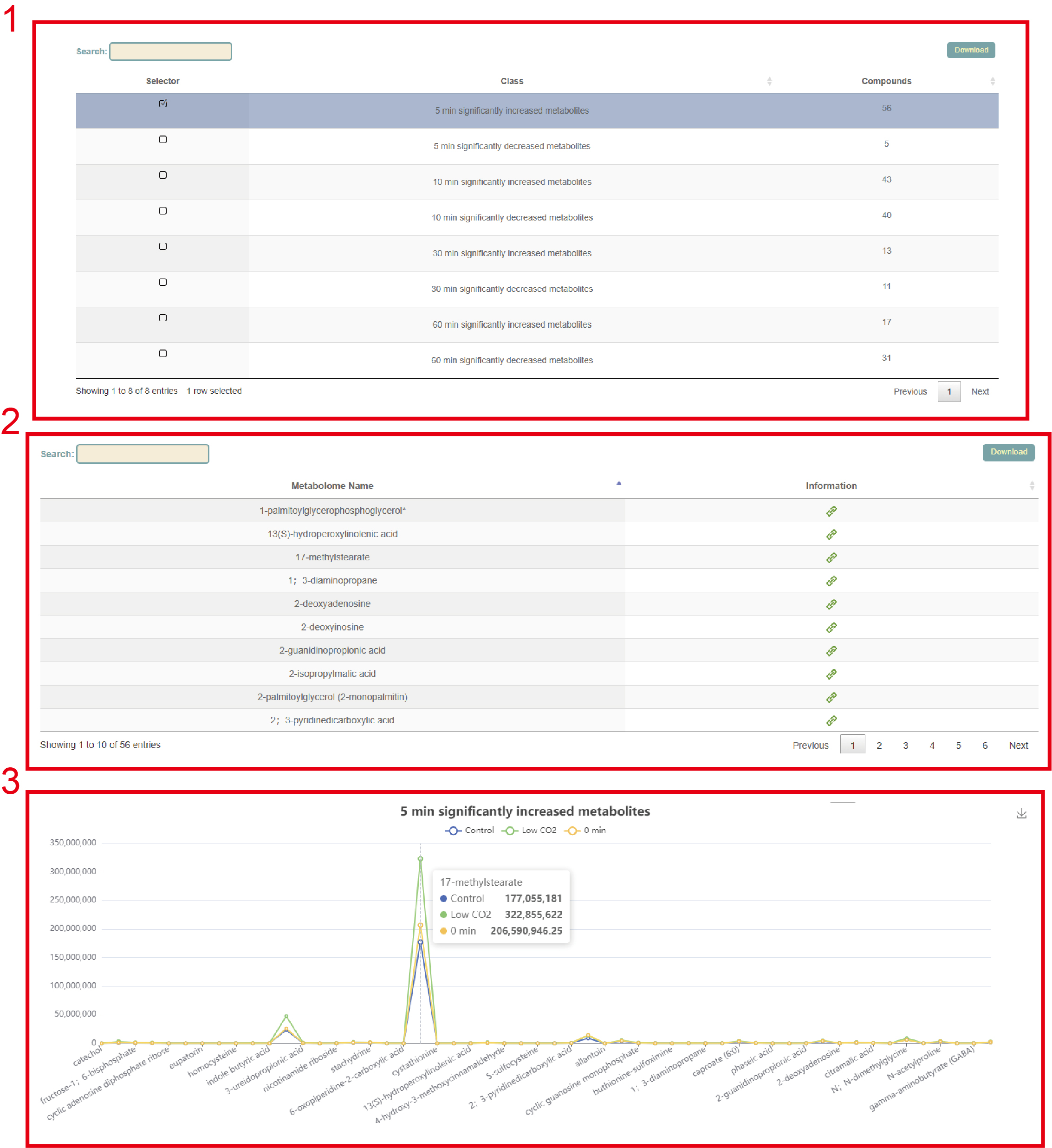
In the metabolome module, we collected data on 544 metabolites from 33 accessions from two studies. According to these two studies, it is divided into two modules, "Guard Cells in Response to Low CO2" and "Laminae and midvein during leaf senescence", where users can search for corresponding sample and metabolite content information respectively. Take the "Guard Cells in Response to Low CO2" module as an example. First, the eight accessions are listed and the user selects the accession to be query at the first column, and then clicks "submit" to submit (box 1). Next, the information of all metabolites of this accession was listed, the user can click the link in the second column to query the relevant information of these metabolites (box 2). Finally, the visualization of the content of different metabolites in the accession, the user can move the mouse to the corresponding point to view the specific value (box 3).
Network
Co-expression
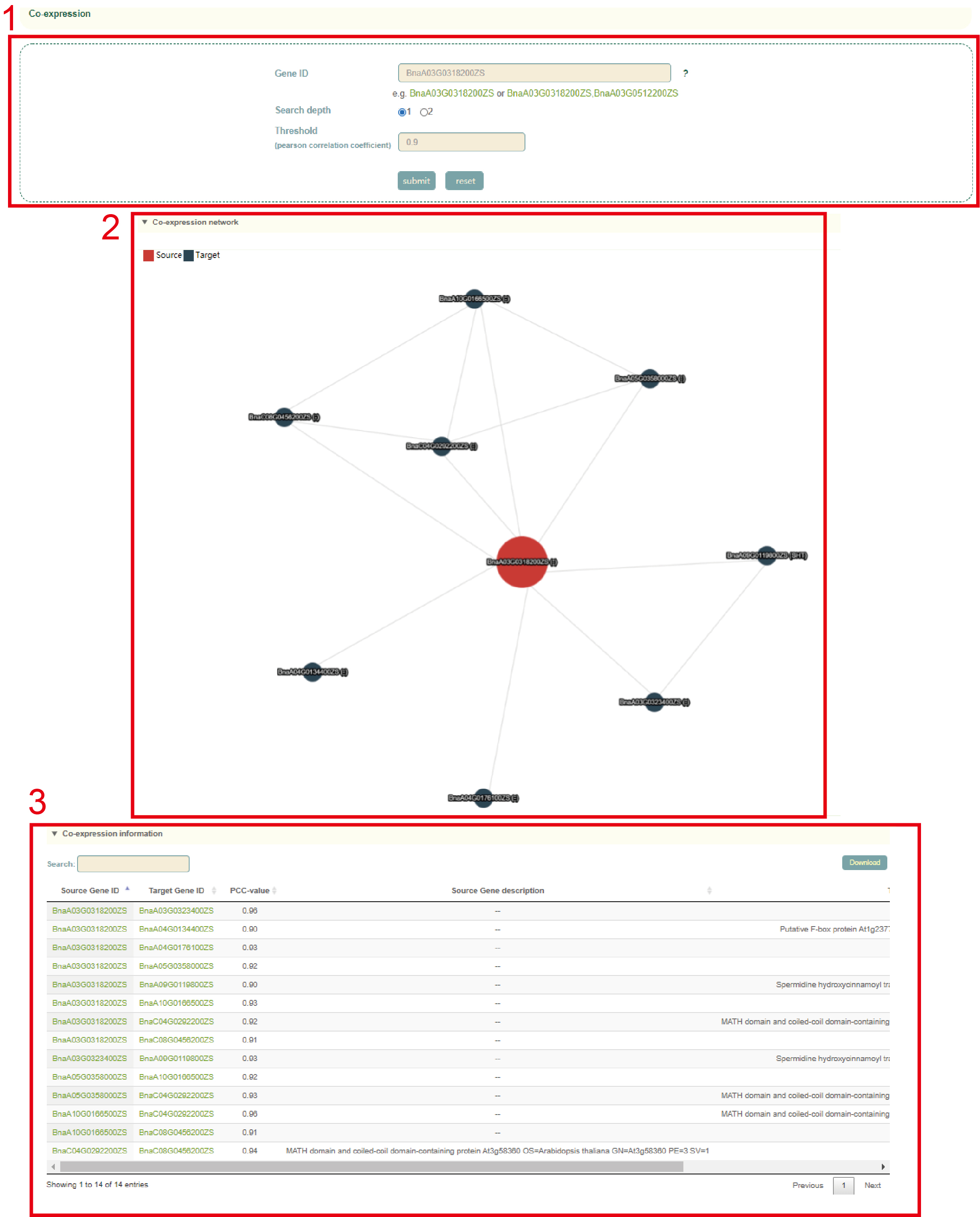
In the Co-expression module, the user first submits one or more gene IDs in the search box, and sets the depth of the network connection (1 or 2) (box 1), and then clicks "submit" to submit. Next, the user will obtain the co-expression network figure of the gene or genes (box 2) and the pearson correlation coefficients and functional information of the gene or genes (box 3).
TF regulation network
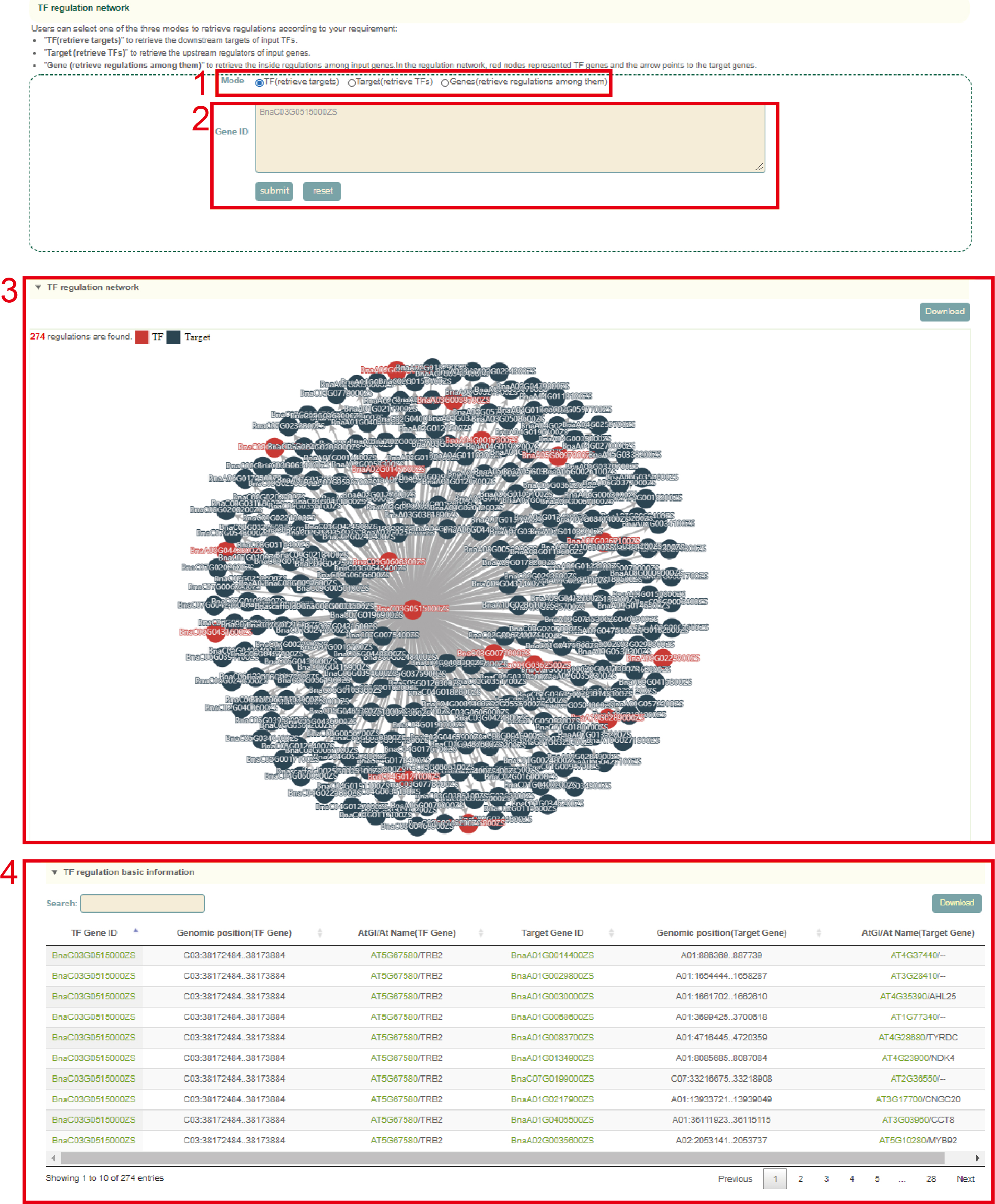
In the TF regulation network module, the user first submits one or more gene IDs (box 1) in the search box, and sets the search modes including TF (to retrieve downstream regulated genes), Target (to retrieve the TF genes) or Genes (to retrieve the TF genes and regulated downstream genes) (box 2), and then clicks "submit" to submit. Next, the user will get the network figure of TFs and the target genes (box 3), the pearson correlation coefficients between them and the function information of the genes (box 4).
Usage of Tools portal
Jbowser
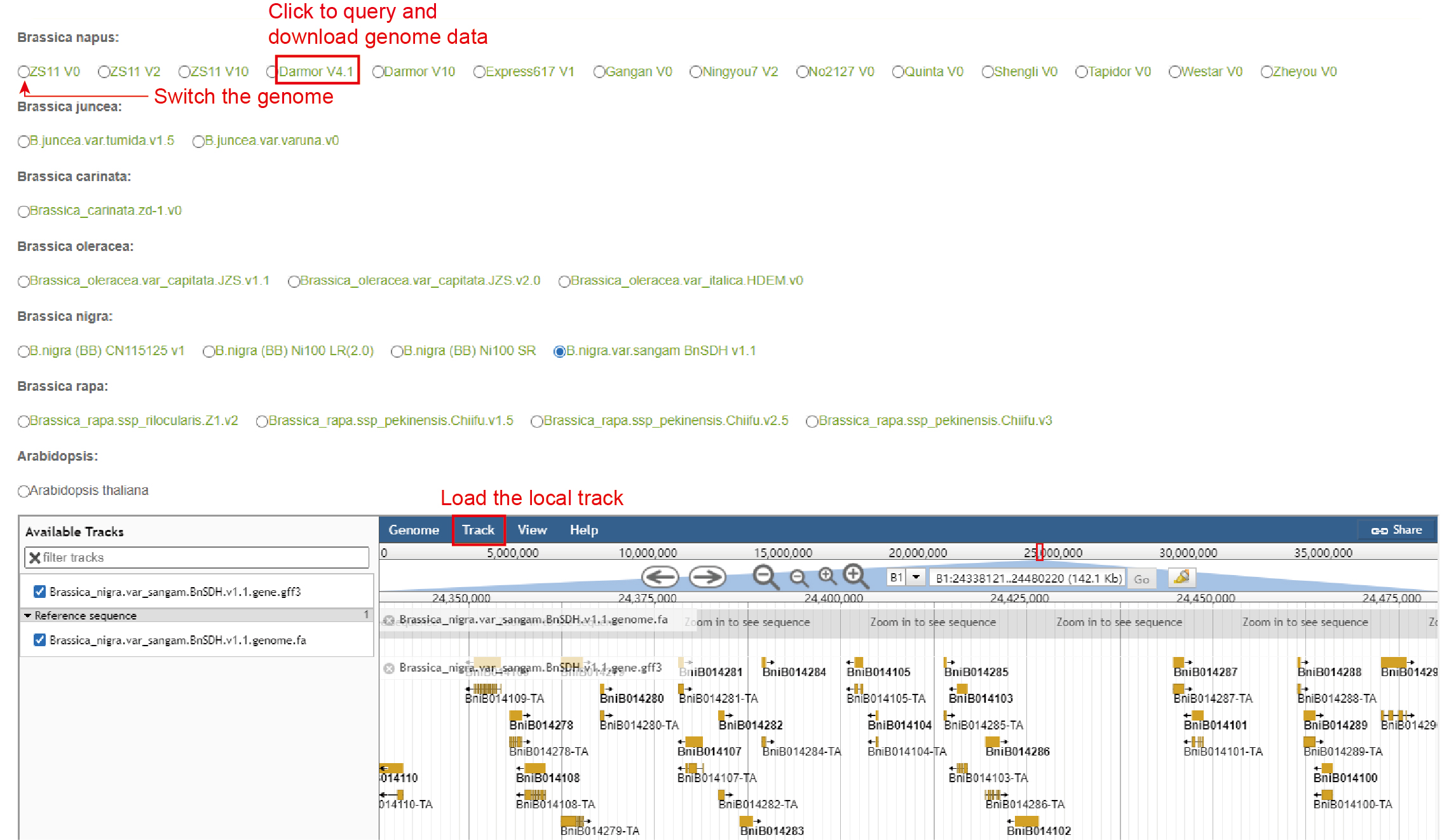
Data: The 29 genome assemblies were provided in Jbowser, including 14 B. napus genome assemblies, 14 other Brassica genome assemblies and A. thaliana genome.
Usage: The user clicks the circle in front of the genome assembly to select the genome, and then in the Jbrowser, the local track file can be uploaded in Track module.
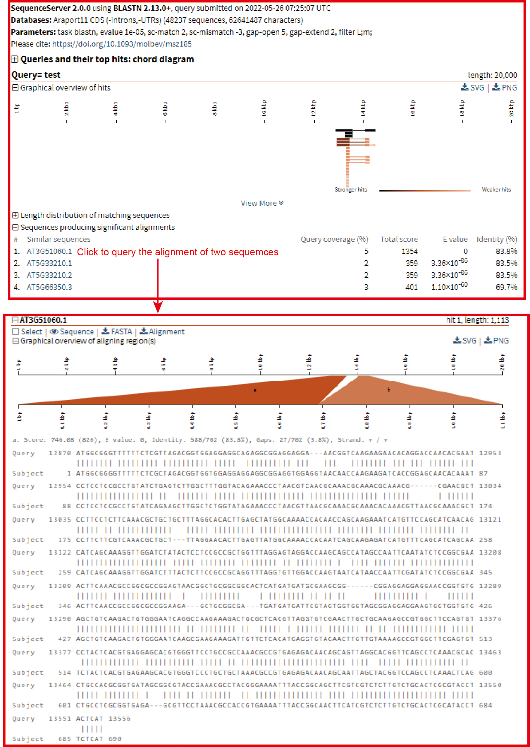
Blast
Data: In Blast, the 15 genome assemblies were provided, including 11 B. napus genome assemblies, another three Brassica genome assemblies and A. thaliana. Their genome, CDS, protein and gene sequences were used to construct the blast library.
Usage:
1. Click the circle in front of the genome assembly and sequence to select the genome and sequence type;
2. Paste the sequence to be queried in the sequence box below;
3. Select the database type and click 'Submit' to submit.
Results:
The first is a graphical representation of the genomic positions to which the sequences are aligned. Then there is a list of all the positions aligned, and the user can click them to query the detailed sequence alignment.

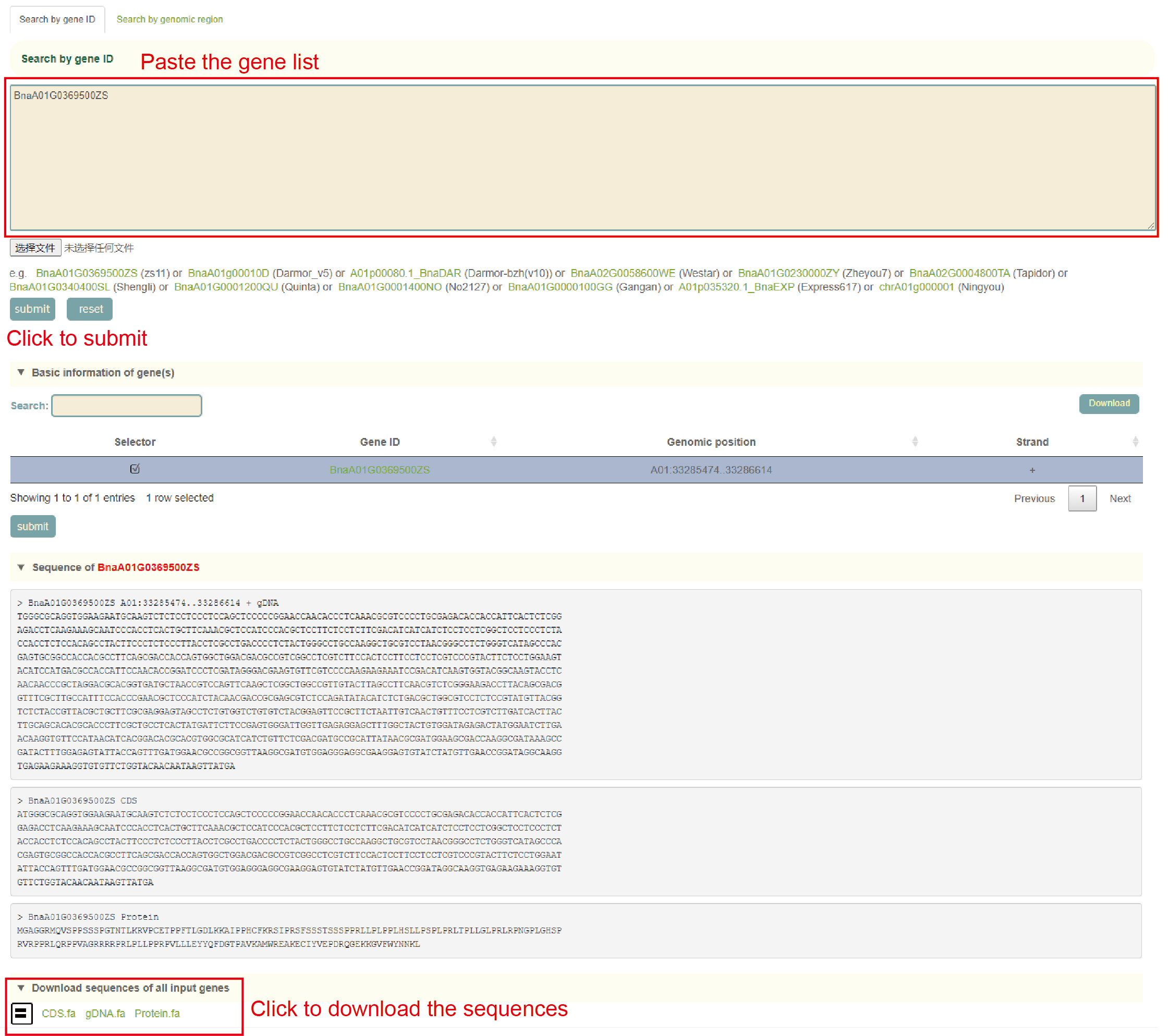
Seq fetch
Usage: Paste the gene list to be aligned in the sequence box or upload the gene list file to be extracted and click "Submit" to submit.
Results: You can directly copy the sequences extracted from the dialog box or click on "CDS", "gDNA" and "Protein" in "Download Sequences of all Input Genes" to download these sequences.
Variation annotation
Usage: Paste the variant data to be aligned in the sequence box or upload the variation file with VCF format to be extracted and click "Submit" to submit.
Results: Click "Variation_annotation.vcf" to download.

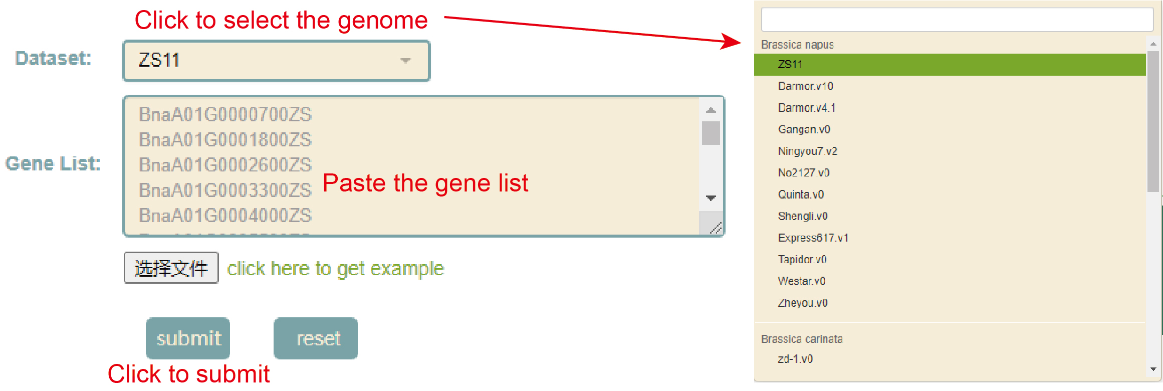
GO enrichment
Usage:
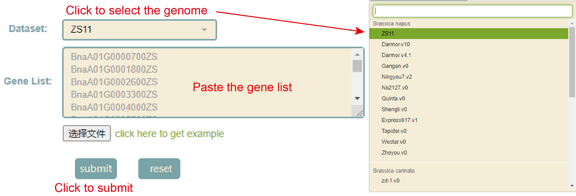
1. Select the genome in "Dataset";
2. Paste the gene list in the sequence box or upload the gene list file, and click Submit;
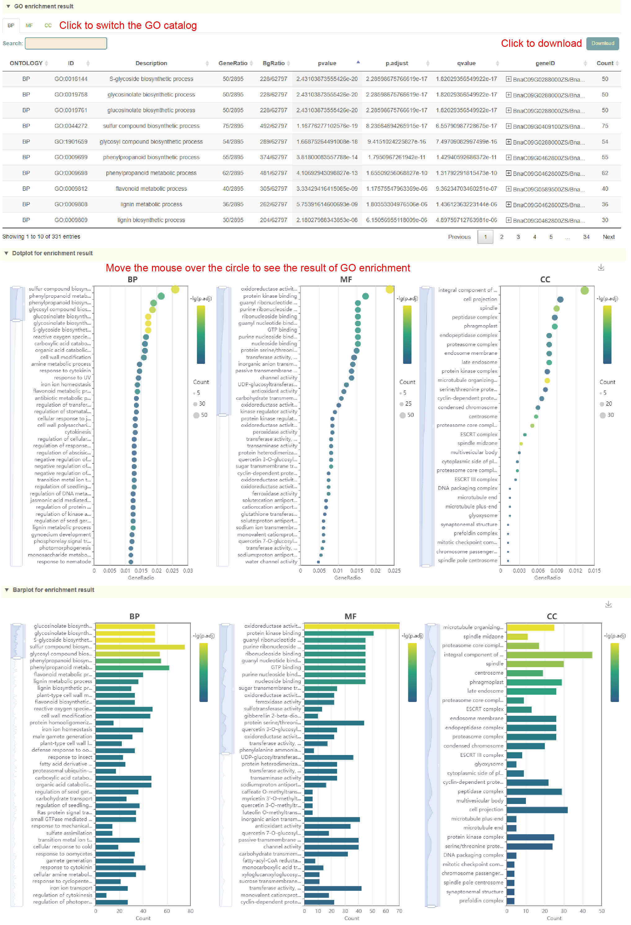
Results:
1. List of results of GO enrichment analysis. You can switch the category of GO by clicking BP, MF and CC above, and click "Download" in the upper right to download;
2. The dot plot and bar plot of GO enrichment analysis results. Move the mouse over the figure to query the statistics of the corresponding GO enrichment analysis results. Click the arrow at the top right to download the image.
KEGG enrichment
Usage:
1. Select the genome in "Dataset";
2. Paste the gene list in the sequence box or upload the gene list file, and click "Submit" to submit;
Results:
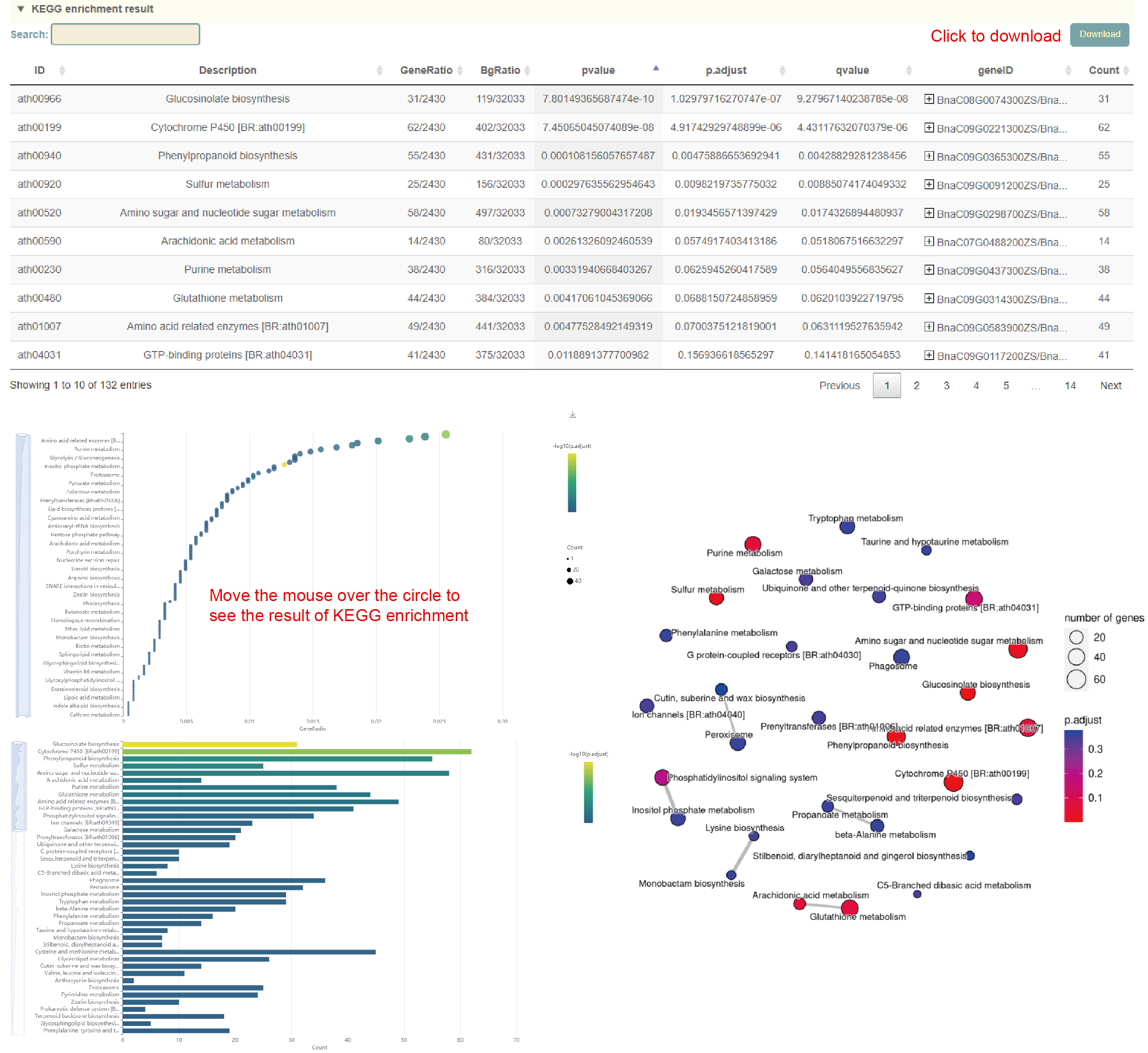
1. The result list of KEGG enrichment analysis. Click "Download" in the upper right to download;
2. Dot plot, bar plot and network plot of KEGG enrichment analysis results. Move the mouse over the figure to query the statistics of the corresponding KEGG enrichment analysis results. Click the arrow at the top right to download the image.
COLOC (Colocalization analysis)
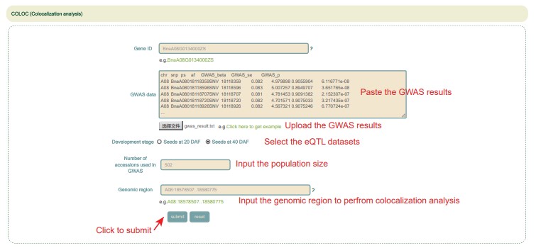
Unlike the COLOC in the Muti-omics module, the COLOC in the Tools module supports user-defined GWAS data. Incidentally, as long as the user has phenotype data, GWAS analysis can also be completed from Online GWAS.
Usage:
1. Enter a ZS11 gene ID.
2. Paste the GWAS result in the GWAS data box or upload the GWAS result file for COLOC.
3. Select the eQTL dataset.
4. Enter the population size used in GWAS analysis.
5. Enter a genomic region less than 1MB and click the submit button.
Results:
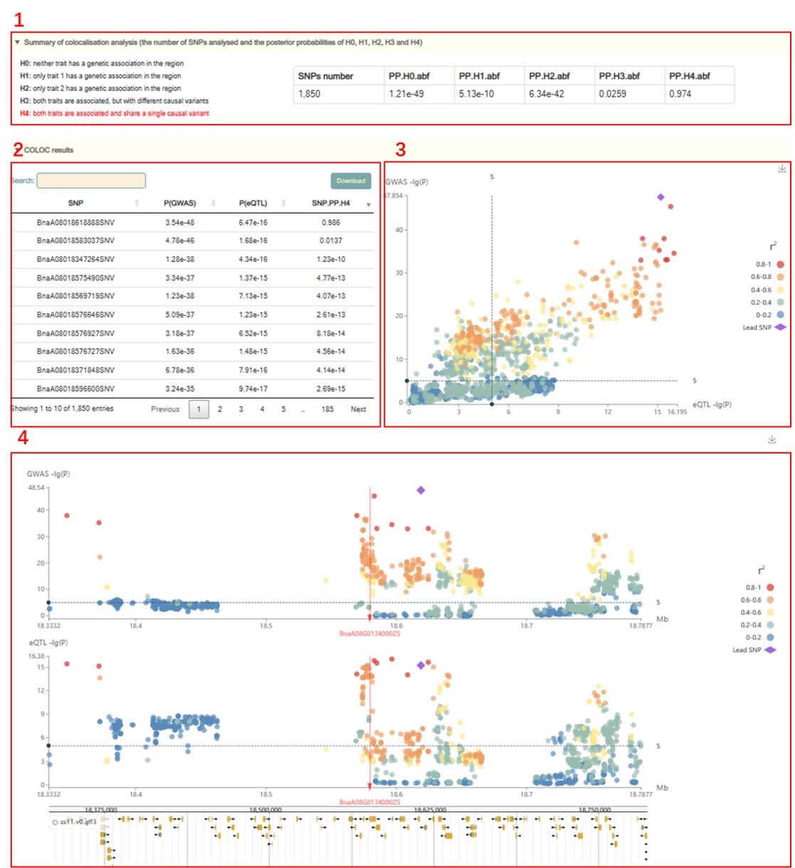
1. The box 1 is main statistics of the results of the co-localization analysis of QTL and eQTL. The red text on the left represents the accepted hypothesis. If the PPH4 value is the largest among all PPH values, the text of the PPH4 hypothesis is marked in red, indicating to accept H4, which is "both traits are associated and share a single causal variant".
2. On the premise of accepting H4, the P-values of GWAS and eQTL and PPH4 values of all variants in this region are listed (box 2), which can be used to locate the causal variation.
3. Users can move the mouse to the figure to browse the detailed statistics of these variants (box 4).
4. Then comes the visualization of the local Manhattan plot of the GWAS and eQTL in the region, and the user can also move the mouse over the points in the plot to see detailed statistics of these variants (box 5). Finally, users can browse the distribution of genetic variation near the gene in the Jbowser browser.
SMR
Unlike the SMR in the Muti-omics module, the SMR in the Tools module supports user-defined GWAS data. Incidentally, as long as the user has phenotype data, GWAS analysis can also be completed from Online GWAS.
Usage:
1. Paste the GWAS result in the GWAS data box or upload the GWAS result file for SMR.
2. Select the eQTL dataset and click the submit button.
Results:
1. The Box 1 shows the SMR analysis results in the form of tables. The result is available if the user clicks the download button.
2. Box 2 visualizes the results of SMR, gwas and eQTL. The red triangle represents lead variation.
SNP match
Usage:
1. Select the genome, ZS11 or Darmor;
2. Paste the genotype data (VCF format) of the sample to be identified in the sequence box or upload the genotype file (VCF format) of the sample and click Submit. SNPmatch will then predict the similarity between the accession to be queried and the 2311 accessions based on the genotype information and output the accessions with a similarity of larger than 0.5.
Results:
1. The result list of SNPmatch: Click "Download" at the top right to download;
2. The bar plot of SNPmatch results, the x axis is the accession name in the population similar to the input accession, and the y axis is the similarity with the sample. Move the mouse to the figure to query the corresponding data. Click the arrow at the top right to download the image.
Primer3
Usage:
1. Enter gene ID, genomic region, gene index, or upload gene list or sequence file;
2. Click "Configure the p3_settings_file" to change the parameters of the configuration file or upload the configuration file;
3. Select the genes to be designed in primers and submit.

Results:
1. The statistical results of primer design: Click "Download" in the upper right to download. Users can select primers for e-PCR alignment;
2. Raw output of Primer3, including visualization of primer sequences and their positions on the genome.
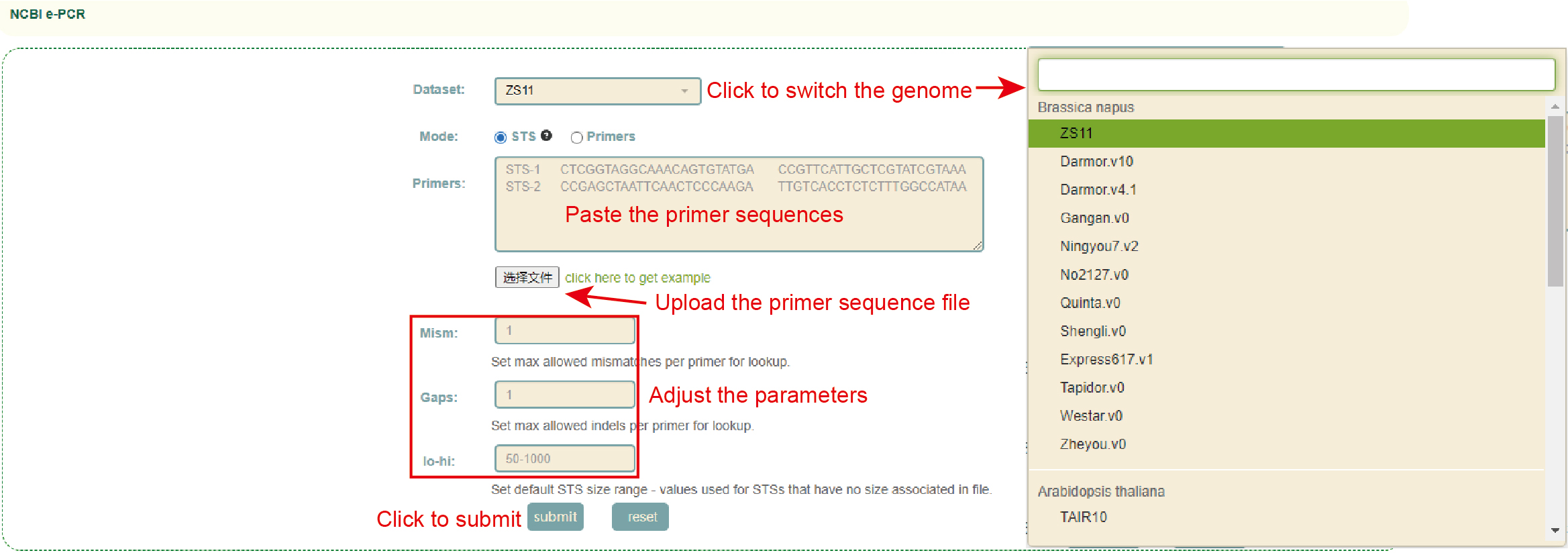
e-PCR
Usage:
1. Click on Dataset to select the genome;
2. Select the file format (STS or Primers) in Mode;
3. Paste the sequence into the dialog or upload the sequence file;
4. Adjust alignment parameters, including mismatch value(mism), gap size(gap) and sequence length range(lo-hi");
5. Click Submit.
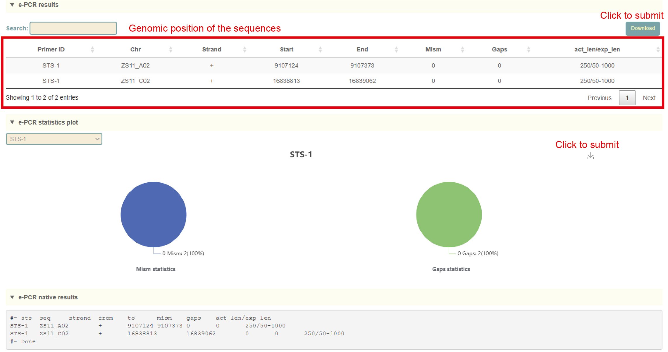
Results:
1. The list of e-PCR results, each row is the position of the sequence amplified by the primers;
2. Statistical chart of e-PCR comparison results, including the ratio of mismatches and gaps;
3. The raw output result of e-PCR.
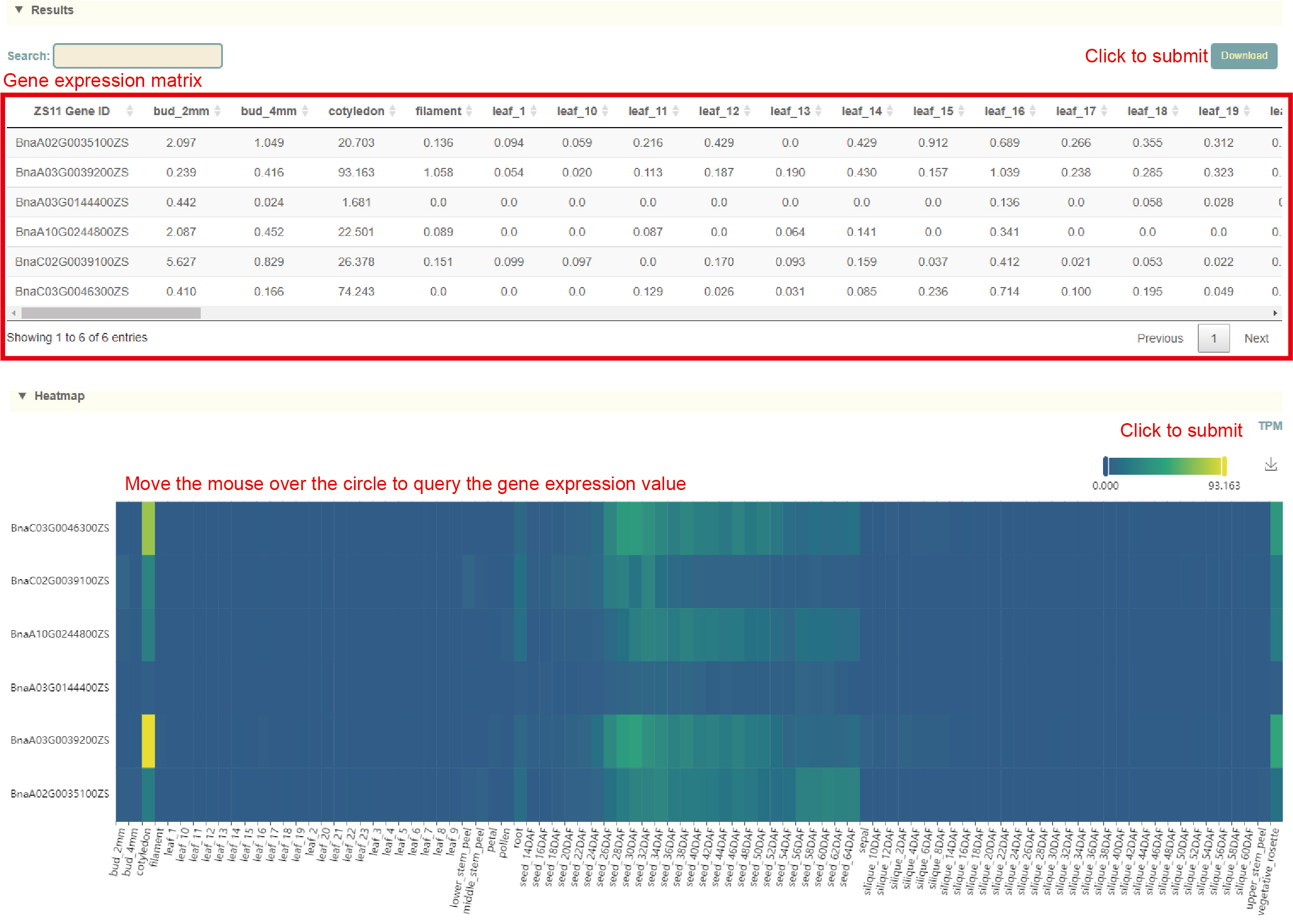
Heatmap
Usage:
1. Paste the gene list to be extracted into the dialog box;
2. Select the RNA-seq dataset, including Tissue, Hormone or Adversity;
3. Select RNA-seq samples and the normalization method for expression levels;
4. Set the parameters of the expression heatmap, such as max, min and colorbar, and click "Submit" to submit.

Results:
1. The gene expression matrix extracted from the list entered by the user and the selected data set can be downloaded by clicking "Download" in the upper right corner;
2. Gene expression quantification heat map drawn. Move the mouse over the graph to view the corresponding values. Click the arrow in the upper right corner to download.
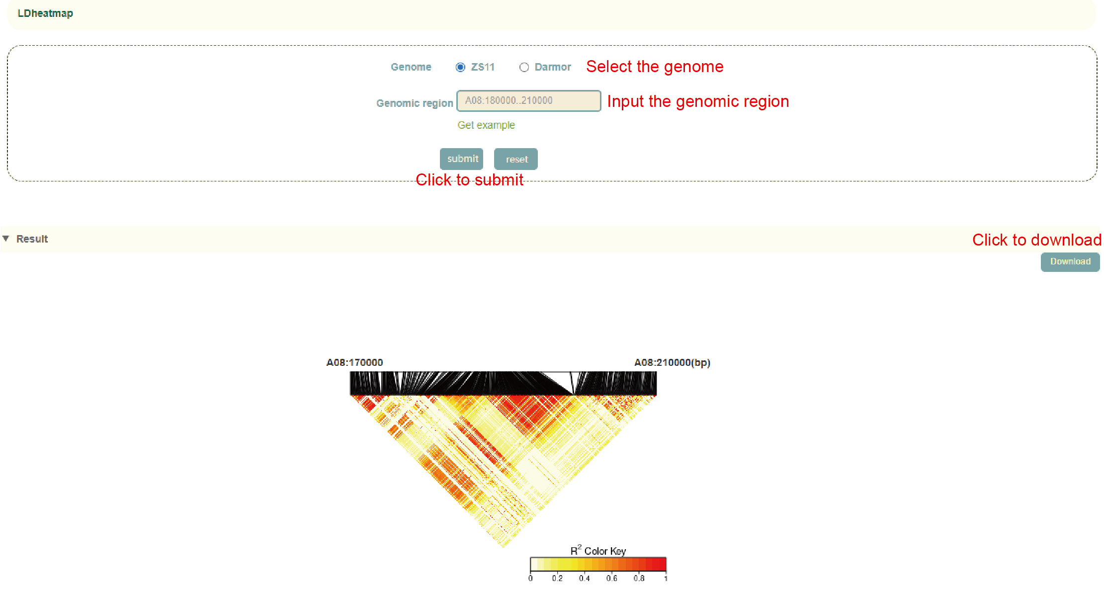
LDheatmap
Usage:
1. Select the genome, ZS11 or Darmor;
2. Enter the genomic region and click 'Submit' to submit.
Results:
Based on user-selected genomes and genomic region, genetic variants are extracted and LD heatmaps are generated. Click "Download" at the top right to download.
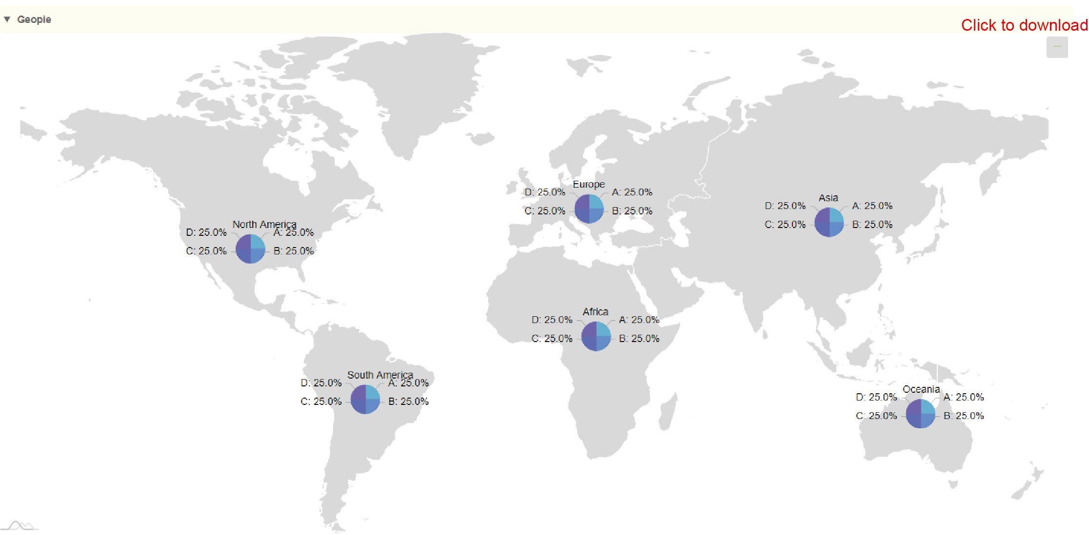
Data2geomap
Usage:
1. Select the image type(Geopie or Geoheatmap);
2. Select the region of the map (World, China or the United States);
3. Enter the drawing data and click "Submit" to submit.
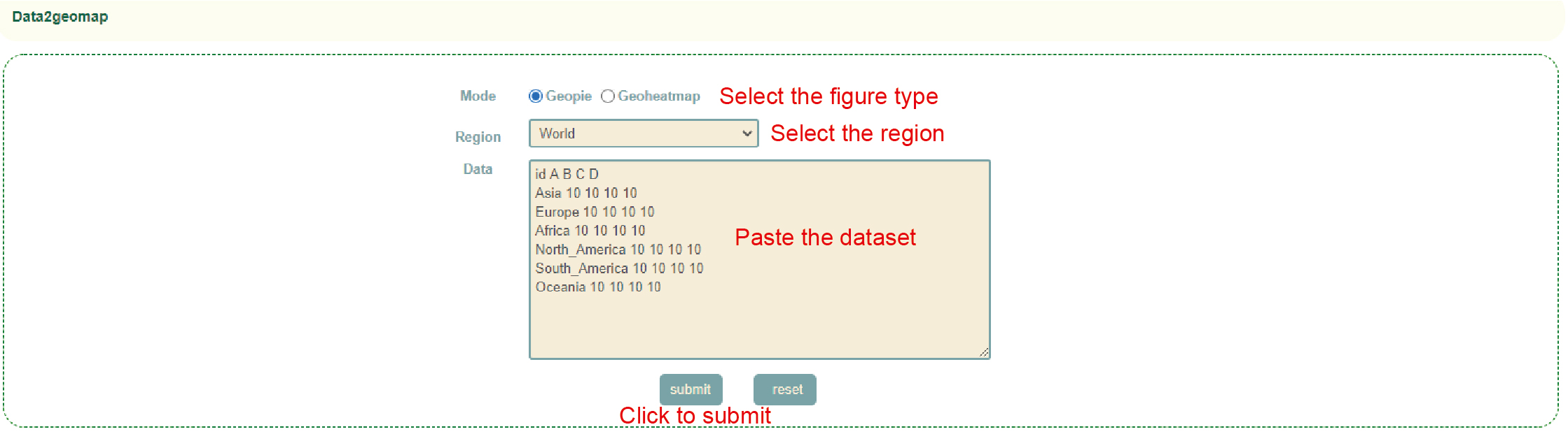
Results:
Generate geographic distribution maps based on user-selected image types, regions, and input data. Click the upper right icon to download.
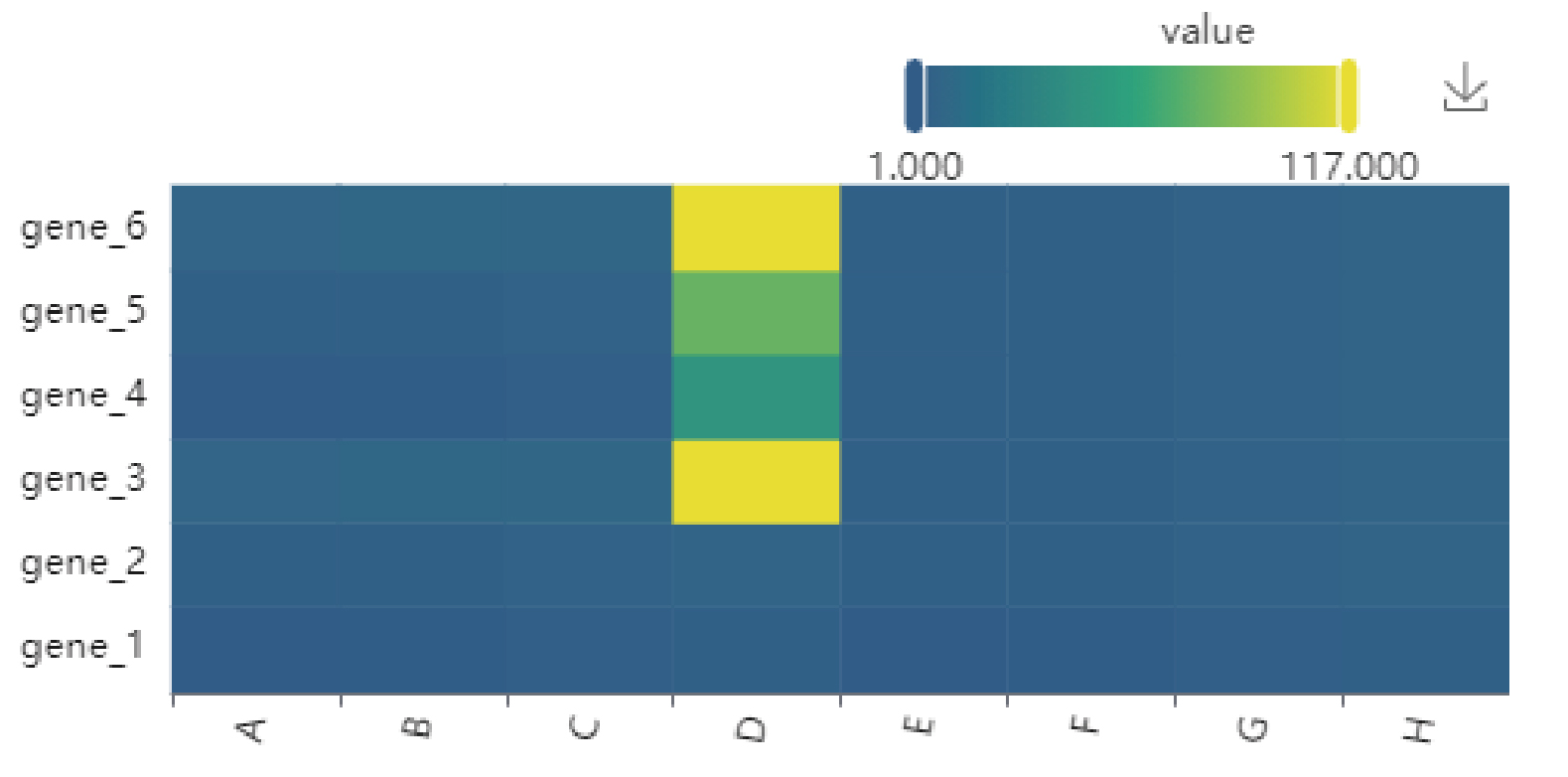
Data2heatmap
Usage:
1. Paste the drawing data into the dialog box or upload the data file;
2. Select the normalization method and drawing parameters and click "Submit" to submit.
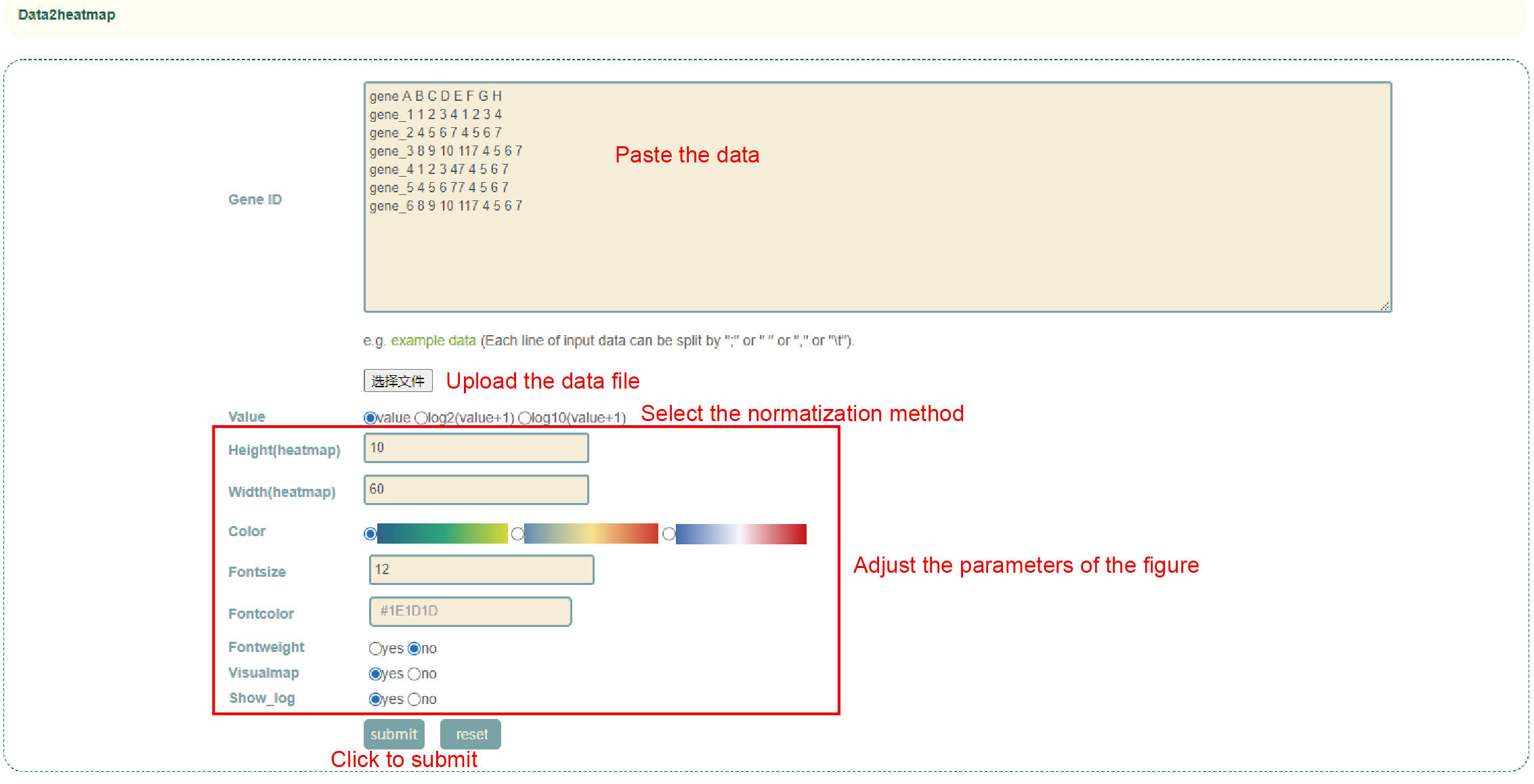
Results:
Generate heatmaps based on user input data and drawing parameters. Click the upper right icon to download.
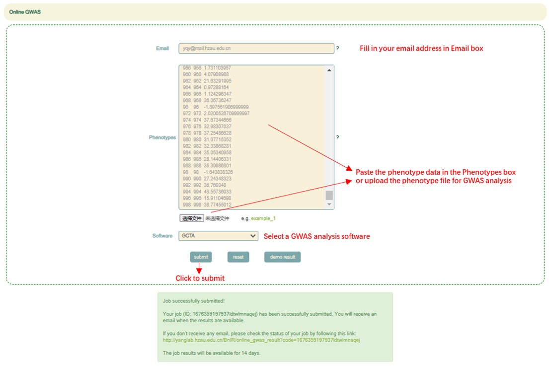
Online GWAS
Usage:
1. Fill in your email address in Email box.
2. Paste the phenotype data in the Phenotypes box or upload the phenotype file for GWAS analysis (The format of the phenotype file must be a table with no header and three columns. The contents of these three columns are: family ID<\t>individual ID<\t>trait. The samples supported by BnIR for GWAS analysis can be found in http://yanglab.hzau.edu.cn/BnIR/population_info).
3. Select a GWAS analysis software in "Software" and click the submit button.
Results:
When the user receives the email or page prompt about the end of work, the user can click the hyperlink in the information prompt to jump to the GWAS result page.

1. The threshold can be adjusted in box 1.
2. Users can click the hyperlink in box 2 to download the original data.
3. Box 3 is a manhattan plot of a 500kb window, in which we denote the p-value of each window by the p-value of the most significant SNP in it. Here, the user can zoom in or out by sliding the mouse wheel, and then move the mouse to the corresponding window to browse the lead SNP and the corresponding p-value in the window.
4. The user can then click on the bars of this window in box 3 to view all the significant SNPs within this region along with the corresponding GWAS statistics (box 4) and Manhattan plots (box 5).